Dynamic Programming Chris Atkeson 2012 Dynamic Programming x

Dynamic Programming Chris Atkeson 2012

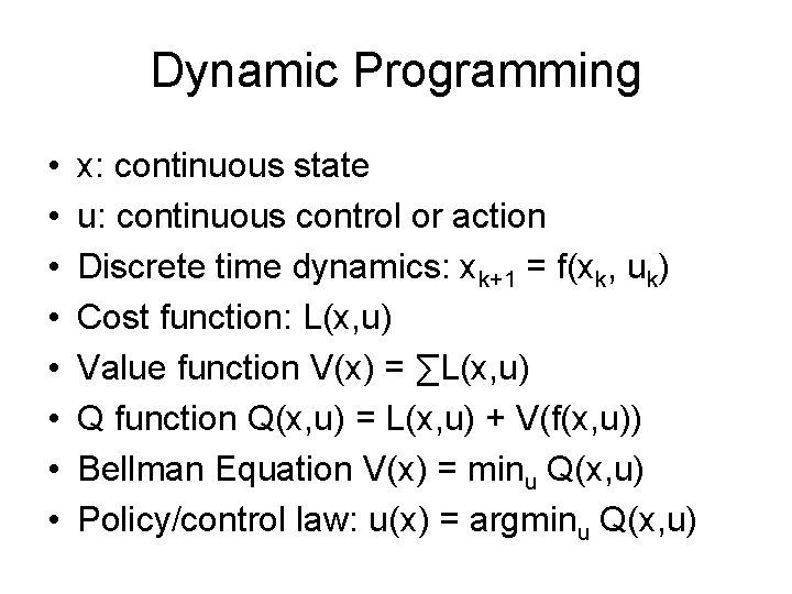
Dynamic Programming • • x: continuous state u: continuous control or action Discrete time dynamics: xk+1 = f(xk, uk) Cost function: L(x, u) Value function V(x) = ∑L(x, u) Q function Q(x, u) = L(x, u) + V(f(x, u)) Bellman Equation V(x) = minu Q(x, u) Policy/control law: u(x) = argminu Q(x, u)

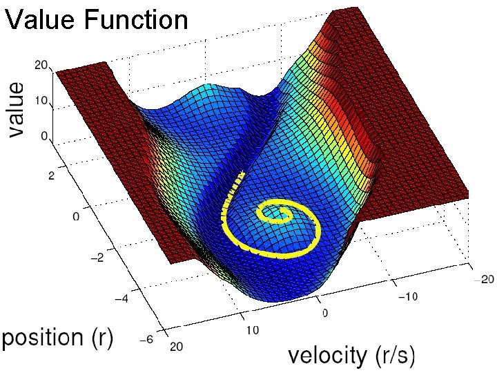
Value Function

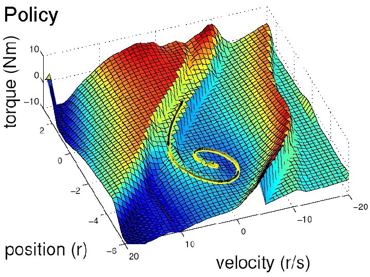
Policy

Why Dynamic Programming? • Trajectory optimization (including receding horizon control) can produce high quality answers. • However, trajectory optimization often gets stuck in local minima that are not useful. • We combine dynamic programming and trajectory optimization to get high quality answers with fewer problems from local minima. DP produces an initial trajectory, which is refined by optimization. • DP produces a policy u(x)

Why Dynamic Programming? • Policy optimization can produce useful answers. • However, need to choose good features/basis functions/parameterization.

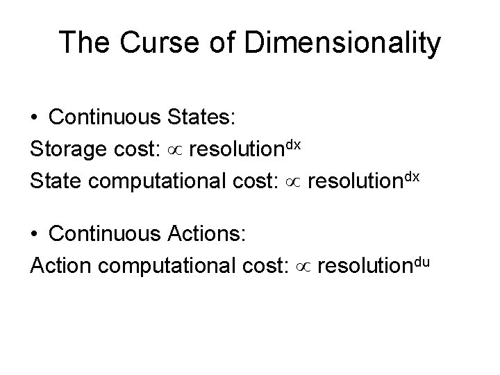
The Curse of Dimensionality • Continuous States: Storage cost: resolutiondx State computational cost: resolutiondx • Continuous Actions: Action computational cost: resolutiondu

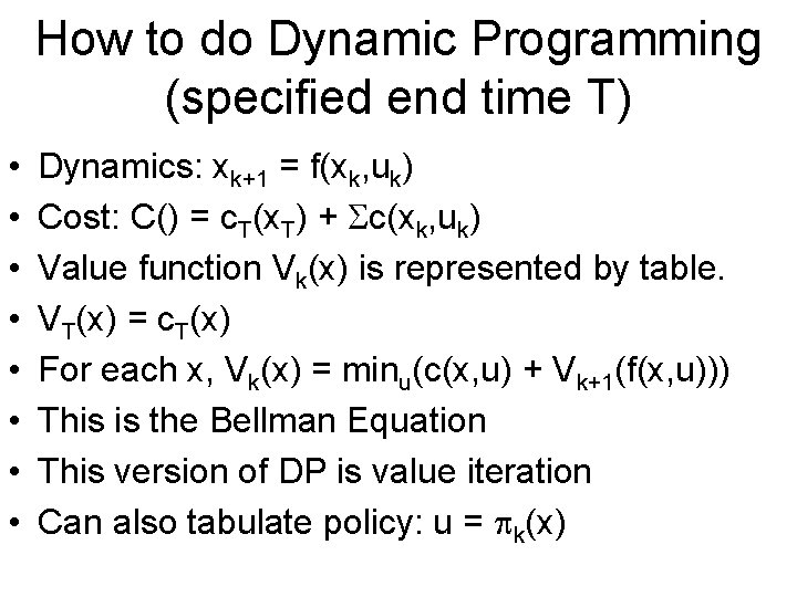
How to do Dynamic Programming (specified end time T) • • Dynamics: xk+1 = f(xk, uk) Cost: C() = c. T(x. T) + c(xk, uk) Value function Vk(x) is represented by table. VT(x) = c. T(x) For each x, Vk(x) = minu(c(x, u) + Vk+1(f(x, u))) This is the Bellman Equation This version of DP is value iteration Can also tabulate policy: u = k(x)

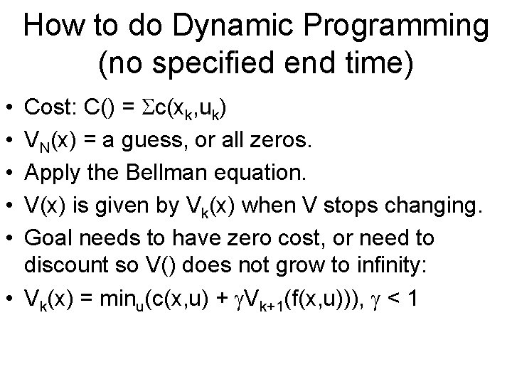
How to do Dynamic Programming (no specified end time) Cost: C() = c(xk, uk) VN(x) = a guess, or all zeros. Apply the Bellman equation. V(x) is given by Vk(x) when V stops changing. Goal needs to have zero cost, or need to discount so V() does not grow to infinity: • Vk(x) = minu(c(x, u) + Vk+1(f(x, u))), < 1 • • •

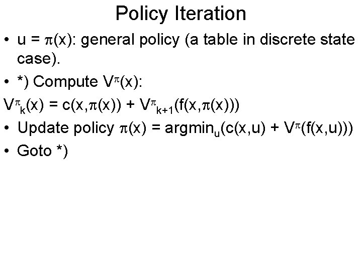
Policy Iteration • u = (x): general policy (a table in discrete state case). • *) Compute V (x): V k(x) = c(x, (x)) + V k+1(f(x, (x))) • Update policy (x) = argminu(c(x, u) + V (f(x, u))) • Goto *)

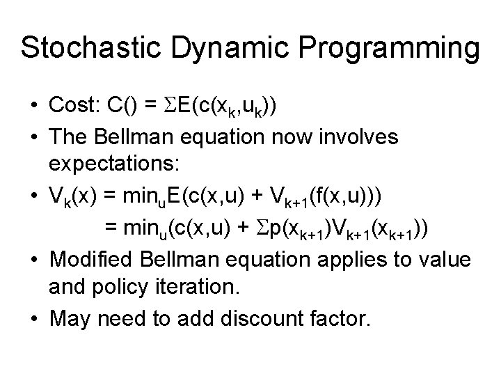
Stochastic Dynamic Programming • Cost: C() = E(c(xk, uk)) • The Bellman equation now involves expectations: • Vk(x) = minu. E(c(x, u) + Vk+1(f(x, u))) = minu(c(x, u) + p(xk+1)Vk+1(xk+1)) • Modified Bellman equation applies to value and policy iteration. • May need to add discount factor.

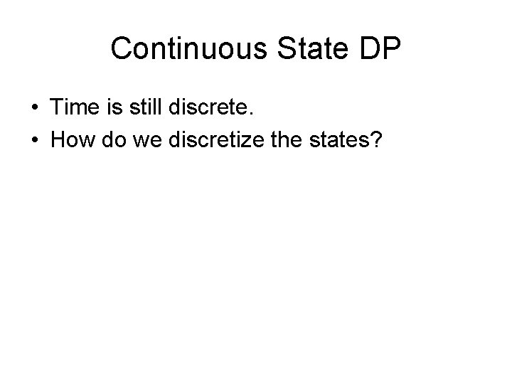
Continuous State DP • Time is still discrete. • How do we discretize the states?

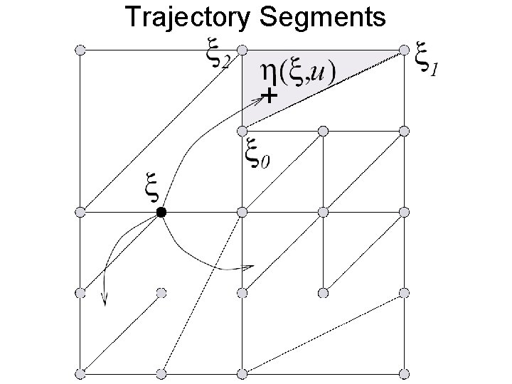
How to handle continuous states. • Discretize states on a grid. • At each point (x 0), generate trajectory segment of length N by minimizing C(u) = c(xk, uk) + V(x. N) • V(x. N): interpolate using surrounding V() • Typically multilinear interpolation used. • N typically determined by when V(x. N) independent of V(x 0) • Use favorite continuous function optimizer to search for best u when minimizing C(u) • Update V() at that cell.

State Increment Dynamic Programming (Larson) c 1 V(x 0) c 0 c 2 V(x. N)

State Increment Dynamic Programming

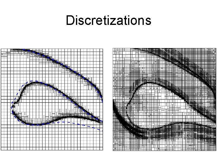
Discretizations • Grid, multilinear interpolation

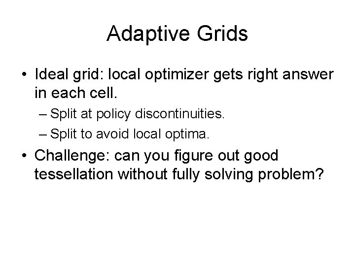
Adaptive Grids • Ideal grid: local optimizer gets right answer in each cell. – Split at policy discontinuities. – Split to avoid local optima. • Challenge: can you figure out good tessellation without fully solving problem?

Munos and Moore, Variable Resolution Discretization in Optimal Control Machine Learning, 49 (2/3), 291 -323, 2002

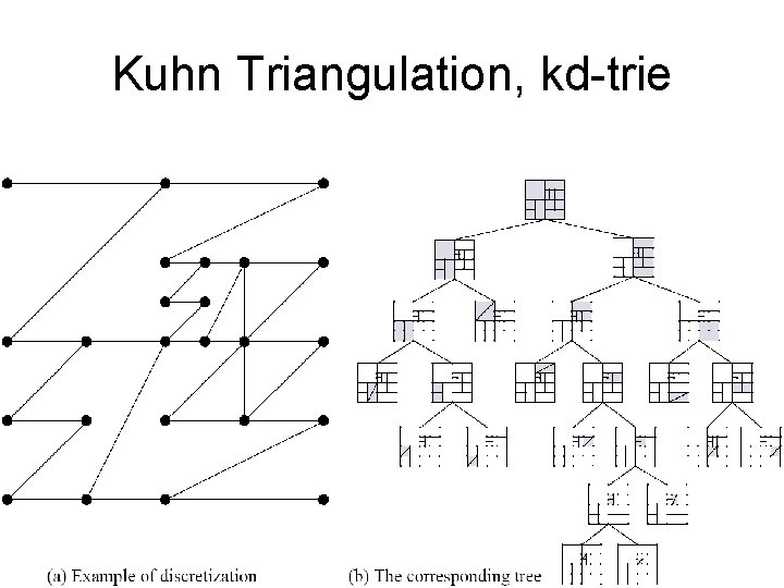
Kuhn Triangulation, kd-trie

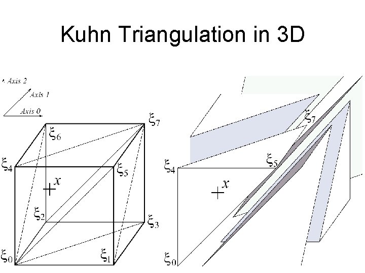
Kuhn Triangulation in 3 D

Trajectory Segments

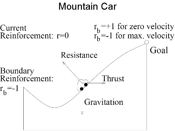
Mountain Car

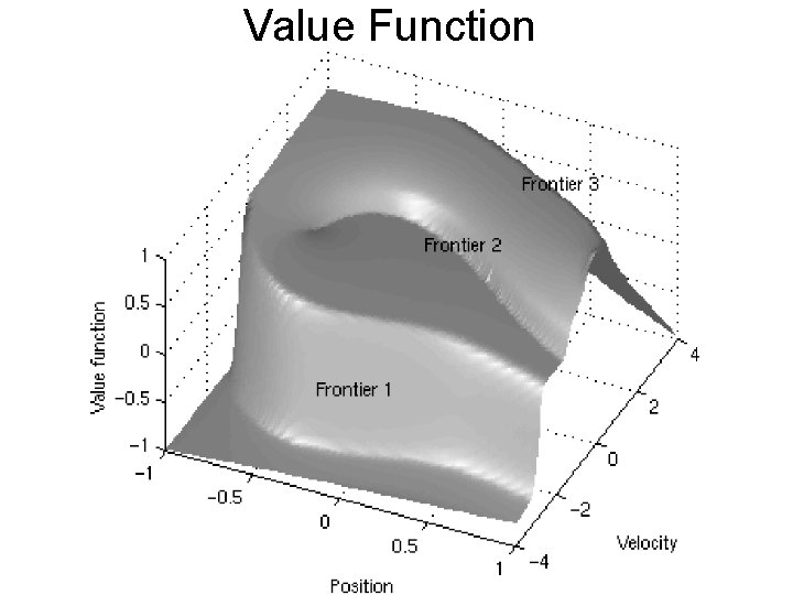
Value Function

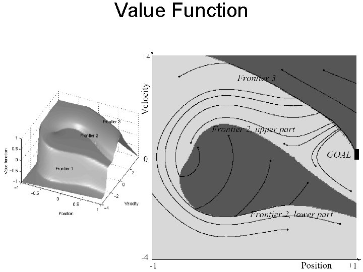
Value Function

Discretizations

Where Split? • Violations of V(x) of cell/region from model (constant, linear, quadratic, …) • Violations of u(x) of cell/region from model (constant, linear, …) • Some criteria applied to predecessors (how much change in V needed to affect trajectory? )

Policy Iteration: Continuous State • • • Discretize states Represent policy at discretized states u(x) Each cell in table has constant u, or u as knot points for linear or higher order spline *) Same kind of trajectory segments used to compute V k(x) = c(x, (x)) + V k+1(x. N) • Optimize policy (x) = argminu(c(x, u) + V (f(x, u))) using favorite continuous function optimizer. • Goto *)

Stochastic DP: Continous State • Cost: C() = E(c(xk, uk)) • Do Monte Carlo sampling of process noise for each trajectory segment (many trajectory segments), or • Propagate analytic distribution (see Kalman filter) • The Bellman equation involves expectations: • Vk(x) = minu. E(c(x, u) + Vk+1(f(x, u)))

Insight • Try to develop planning methods that scale computational cost according to complexity of problem. • Simple problems are easy to solve (LQR) • Complicated problems are expensive to solve, or aren’t solvable with current methods.

Ideas • • • Randomly sample actions Randomly sample states Use local models Propagate local models along trajectories Locally optimize Coordinate local optimizations to globally optimize.

What about continuous actions?

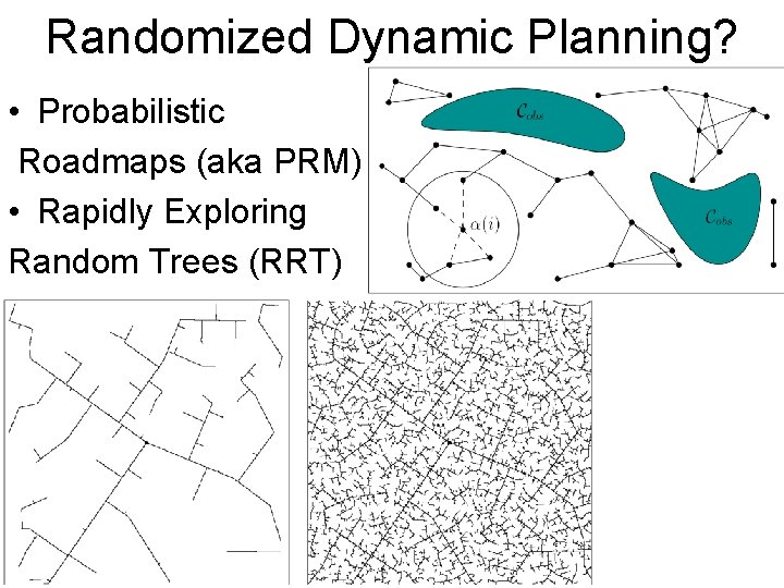
Randomized Dynamic Planning? • Probabilistic Roadmaps (aka PRM) • Rapidly Exploring Random Trees (RRT)

Random Sampling DP: Related Work • Semi-uniform strategies in multi-armed bandit problems: Epsilon-X strategies. • Evolutionary (random) action search. • Nemirovsky and Yudin: can’t beat curse of dimensionality in continuous action search. • Rust 97: Random sampling of states in stochastic DP. E() smooths problem. Beat curse of dimensionality for computing E(). • Thrun 00: POMDPs. Random sampling of belief states. Nearest neighbor interpolation of V(). Coverage vs. surprise test.

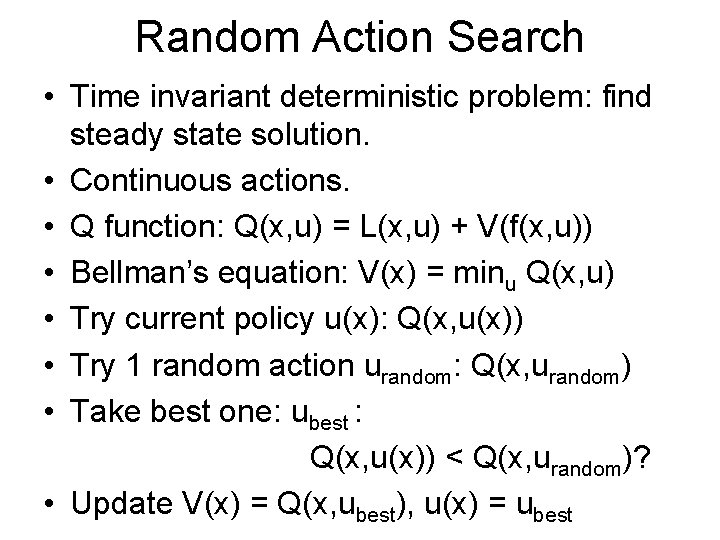
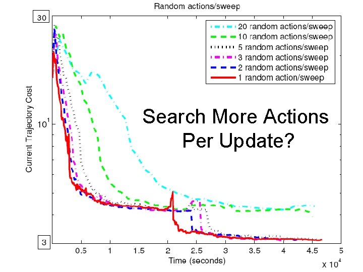
Random Action Search • Time invariant deterministic problem: find steady state solution. • Continuous actions. • Q function: Q(x, u) = L(x, u) + V(f(x, u)) • Bellman’s equation: V(x) = minu Q(x, u) • Try current policy u(x): Q(x, u(x)) • Try 1 random action urandom: Q(x, urandom) • Take best one: ubest : Q(x, u(x)) < Q(x, urandom)? • Update V(x) = Q(x, ubest), u(x) = ubest

DP Asynchronous

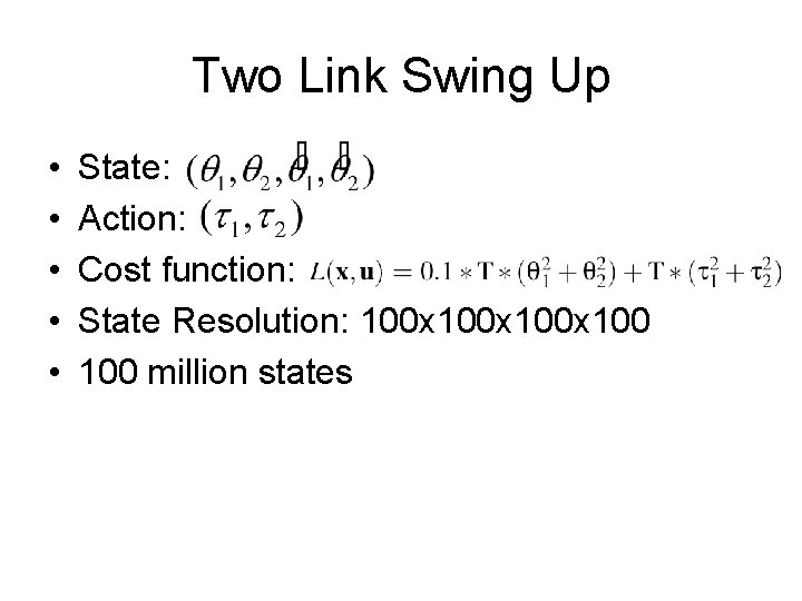
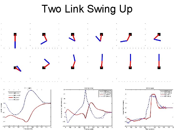
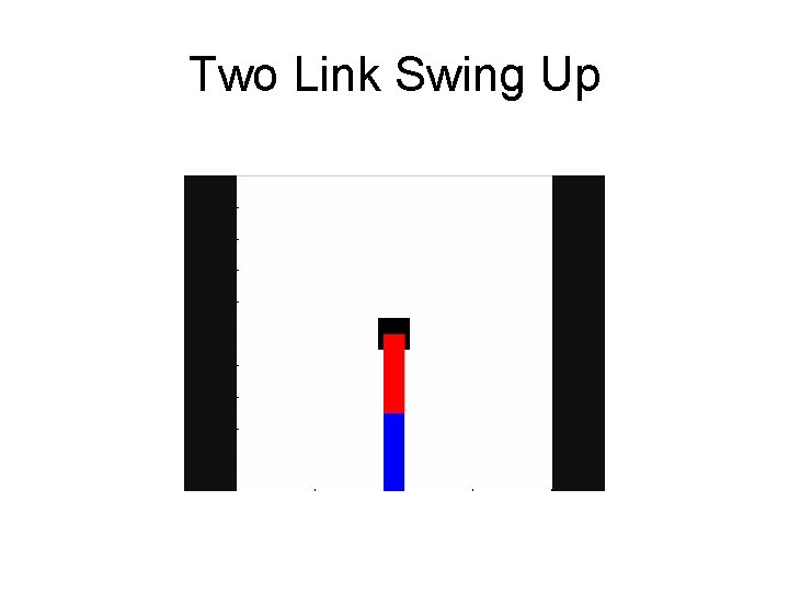
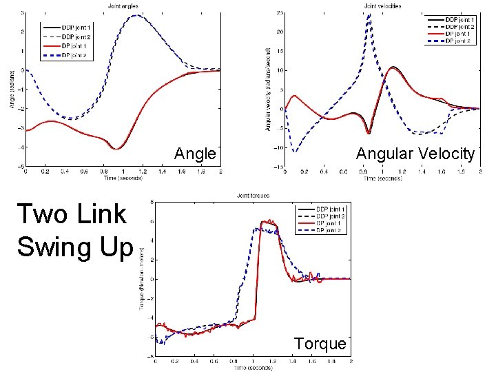
Two Link Swing Up • • • State: Action: Cost function: State Resolution: 100 x 100 million states

Two Link Swing Up

Two Link Swing Up

Angle Angular Velocity Two Link Swing Up Torque

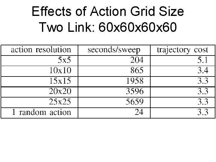
Effects of Action Grid Size Two Link: 60 x 60 x 60

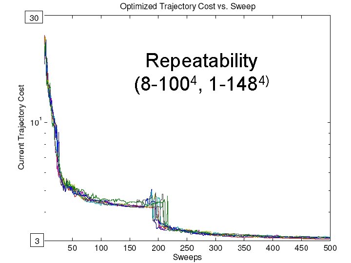
Repeatability (8 -1004, 1 -1484)

Search More Actions Per Update?

Random Sampling of Actions: Improvements • Tune distribution to problem. • Do some local optimization (gradient descent): so far only slows search down. • Smooth output trajectory with trajectory optimization. • Schedule updates adaptively