Dynamic Programming Carrie Williams What is Dynamic Programming

Dynamic Programming Carrie Williams

What is Dynamic Programming? Method of breaking the problem into smaller, simpler sub-problems n Start with the smallest sub-problems and combine to produce a solution n Similar to Divide and Conquer n – But uses a bottom-top approach

When is it used? Most often used with Optimization Problems n When the Brute Force approach becomes too time consuming n – Brute Force is when you find all possible solutions and compare them

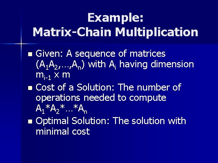
Example: Matrix-Chain Multiplication Given: A sequence of matrices (A 1 A 2, …, An) with Ai having dimension mi-1 x m n Cost of a Solution: The number of operations needed to compute A 1*A 2*…*An n Optimal Solution: The solution with minimal cost n

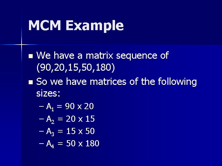
MCM Example We have a matrix sequence of (90, 20, 15, 50, 180) n So we have matrices of the following sizes: n – A 1 = 90 x 20 – A 2 = 20 x 15 – A 3 = 15 x 50 – A 4 = 50 x 180

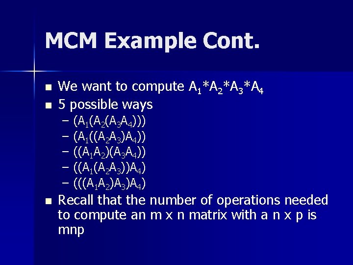
MCM Example Cont. n n We want to compute A 1*A 2*A 3*A 4 5 possible ways – – – n (A 1(A 2(A 3 A 4))) (A 1((A 2 A 3)A 4)) ((A 1 A 2)(A 3 A 4)) ((A 1(A 2 A 3))A 4) (((A 1 A 2)A 3)A 4) Recall that the number of operations needed to compute an m x n matrix with a n x p is mnp

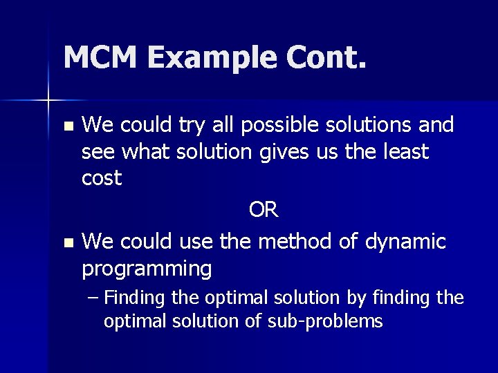
MCM Example Cont. We could try all possible solutions and see what solution gives us the least cost OR n We could use the method of dynamic programming n – Finding the optimal solution by finding the optimal solution of sub-problems

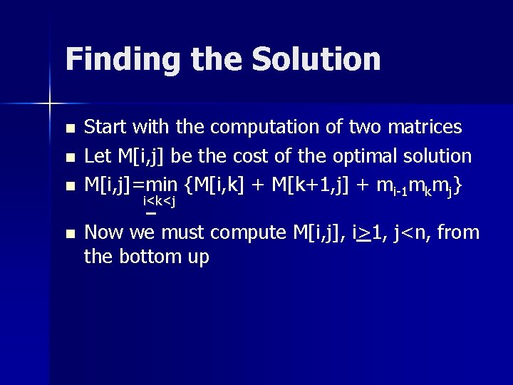
Finding the Solution n n Start with the computation of two matrices Let M[i, j] be the cost of the optimal solution M[i, j]=min {M[i, k] + M[k+1, j] + mi-1 mkmj} i<k<j Now we must compute M[i, j], i>1, j<n, from the bottom up

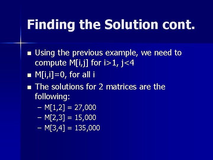
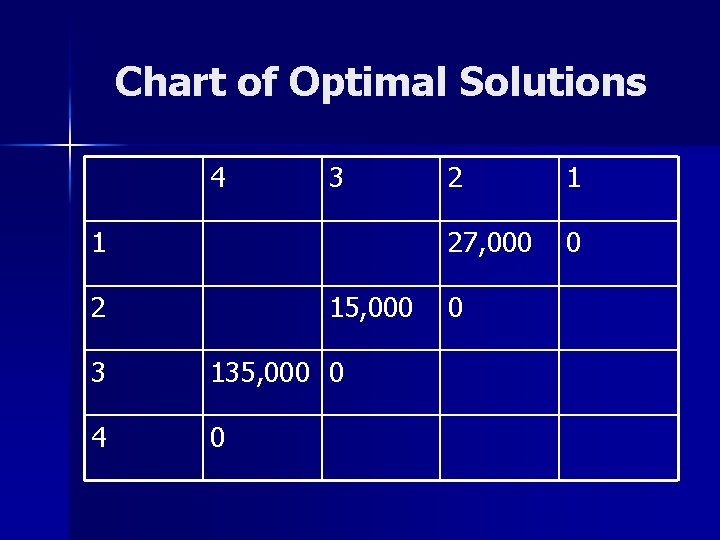
Finding the Solution cont. n n n Using the previous example, we need to compute M[i, j] for i>1, j<4 M[i, i]=0, for all i The solutions for 2 matrices are the following: – – – M[1, 2] = 27, 000 M[2, 3] = 15, 000 M[3, 4] = 135, 000

Chart of Optimal Solutions 4 3 1 2 15, 000 3 135, 000 0 4 0 2 1 27, 000 0 0

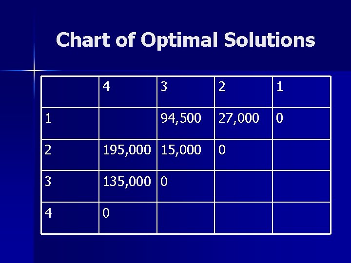
Computing the Cost of Three Matrices n n M[1, 3] = min {M[1, 2] + M[3, 3] + m 0 m 2 m 3} {M[1, 1] + M[2, 3] + m 0 m 1 m 3} = 27, 000 + 90*15*50 = 94, 500 = 0 + 15, 000 + 90*20*50 = 105, 000 M[2, 4] = min {M[2, 3] + M[4, 4] + m 1 m 3 m 4} {M[2, 2] + M[3, 4] + m 1 m 2 m 4} = 15, 000 + 20*50*180 = 195, 000 = 0 + 135, 000 + 20*50*180 = 315, 000 Minimum for M[1, 3] = 94, 500 = ((A 1 A 2)A 3) Minimum for M[2, 4] = 195, 000 = (A 2(A 3 A 4))

Chart of Optimal Solutions 4 3 2 1 1 94, 500 27, 000 0 2 195, 000 15, 000 3 135, 000 0 4 0 0

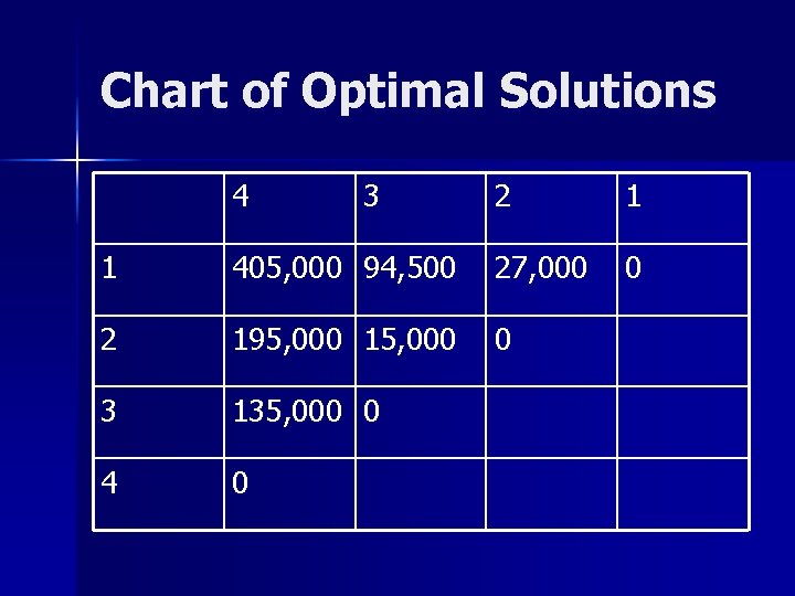
Computing the Cost of Four Matrices n n M[1, 4] = min {M[1, 3] + M[4, 4] +m 0 m 3 m 4} {M[1, 2] + M[3, 4] + m 0 m 2 m 4} {M[1, 1] + M[2, 4] + m 0 m 1 m 4} = 94, 500 + 90*50*180 = 904, 000 = 27, 000 + 135, 000 +90*15*180=405, 000 = 0 + 195, 000 + 90*20*180 = 519, 000 Hence, the minimum cost is 405, 000, which is ((A 1 A 2)(A 3 A 4))

Chart of Optimal Solutions 4 3 2 1 0 1 405, 000 94, 500 27, 000 2 195, 000 15, 000 0 3 135, 000 0 4 0

Conclusion n n We used the method of dynamic programming to solve the matrix-chain multiplication problem We broke the problem into three subproblems – The minimal cost of two matrices, then three matrices, and finally four matrices n We found the solution by using the subproblem’s optimal solutions