Dynamic Programming An algorithm design paradigm like divideandconquer

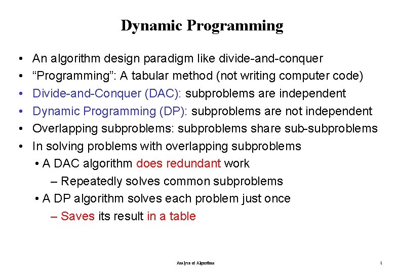
Dynamic Programming • • • An algorithm design paradigm like divide-and-conquer “Programming”: A tabular method (not writing computer code) Divide-and-Conquer (DAC): subproblems are independent Dynamic Programming (DP): subproblems are not independent Overlapping subproblems: subproblems share sub-subproblems In solving problems with overlapping subproblems • A DAC algorithm does redundant work – Repeatedly solves common subproblems • A DP algorithm solves each problem just once – Saves its result in a table Analysis of Algorithms 1

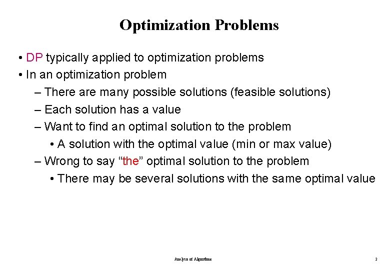
Optimization Problems • DP typically applied to optimization problems • In an optimization problem – There are many possible solutions (feasible solutions) – Each solution has a value – Want to find an optimal solution to the problem • A solution with the optimal value (min or max value) – Wrong to say “the” optimal solution to the problem • There may be several solutions with the same optimal value Analysis of Algorithms 2

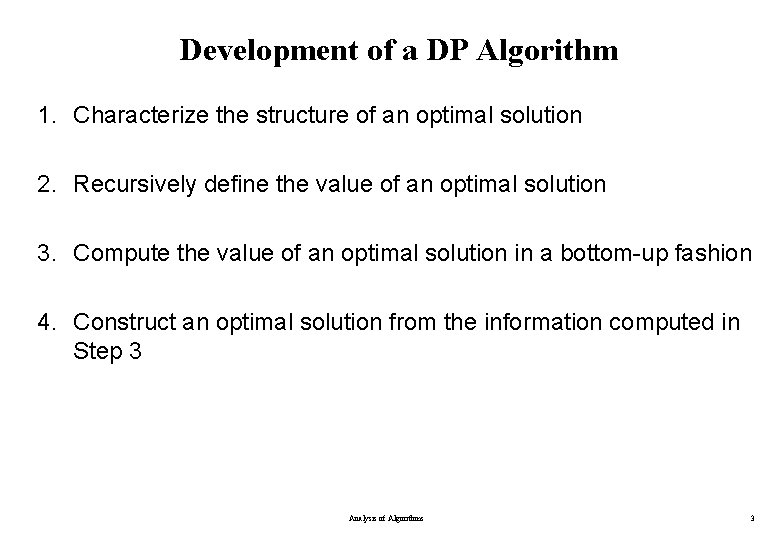
Development of a DP Algorithm 1. Characterize the structure of an optimal solution 2. Recursively define the value of an optimal solution 3. Compute the value of an optimal solution in a bottom-up fashion 4. Construct an optimal solution from the information computed in Step 3 Analysis of Algorithms 3

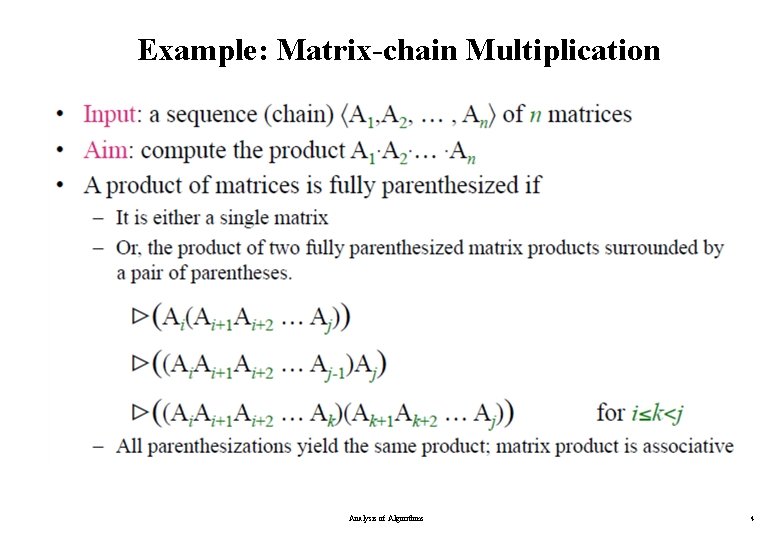
Example: Matrix-chain Multiplication Analysis of Algorithms 4

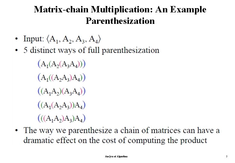
Matrix-chain Multiplication: An Example Parenthesization Analysis of Algorithms 5

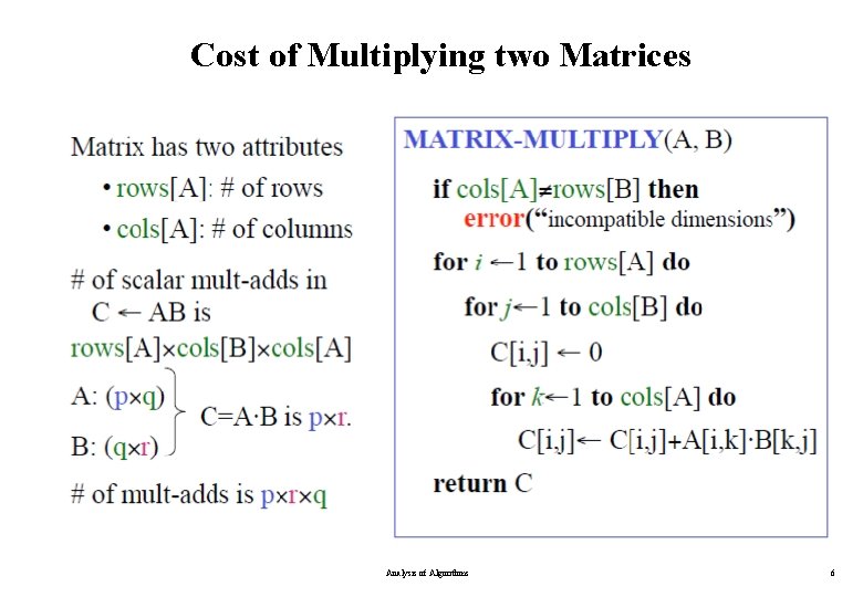
Cost of Multiplying two Matrices Analysis of Algorithms 6

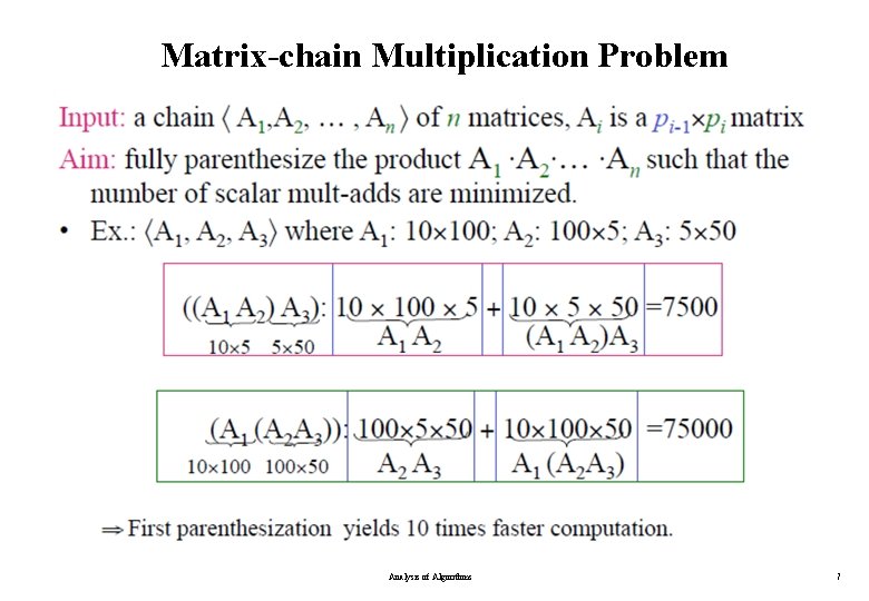
Matrix-chain Multiplication Problem Analysis of Algorithms 7

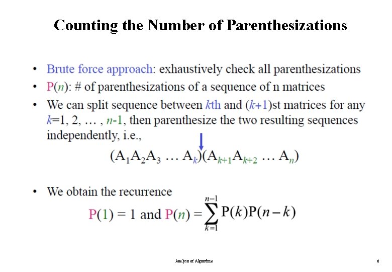
Counting the Number of Parenthesizations Analysis of Algorithms 8

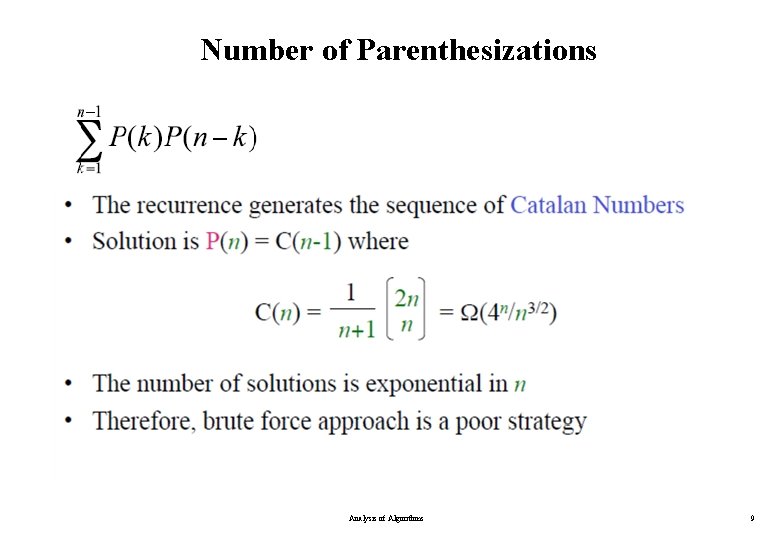
Number of Parenthesizations Analysis of Algorithms 9

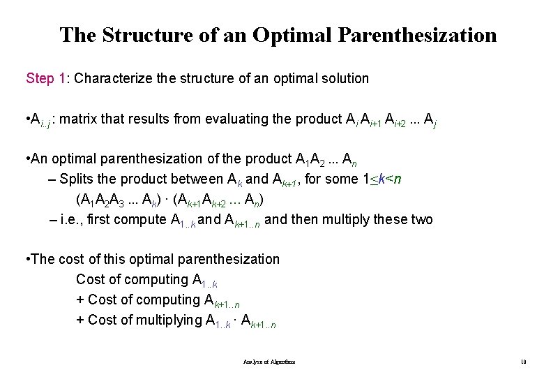
The Structure of an Optimal Parenthesization Step 1: Characterize the structure of an optimal solution • Ai. . j : matrix that results from evaluating the product Ai Ai+1 Ai+2. . . Aj • An optimal parenthesization of the product A 1 A 2. . . An – Splits the product between Ak and Ak+1, for some 1≤k<n (A 1 A 2 A 3. . . Ak) · (Ak+1 Ak+2. . . An) – i. e. , first compute A 1. . k and Ak+1. . n and then multiply these two • The cost of this optimal parenthesization Cost of computing A 1. . k + Cost of computing Ak+1. . n + Cost of multiplying A 1. . k · Ak+1. . n Analysis of Algorithms 10

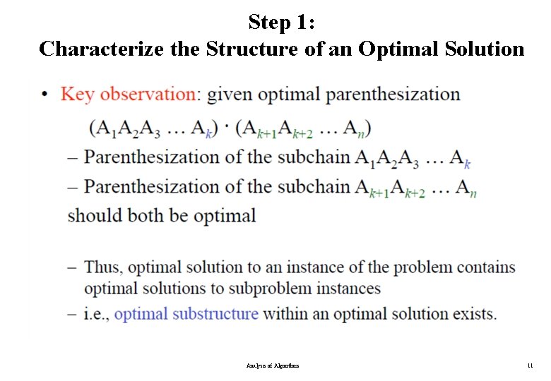
Step 1: Characterize the Structure of an Optimal Solution Analysis of Algorithms 11

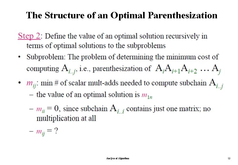
The Structure of an Optimal Parenthesization Analysis of Algorithms 12

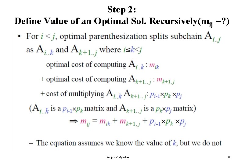
Step 2: Define Value of an Optimal Sol. Recursively(mij =? ) Analysis of Algorithms 13

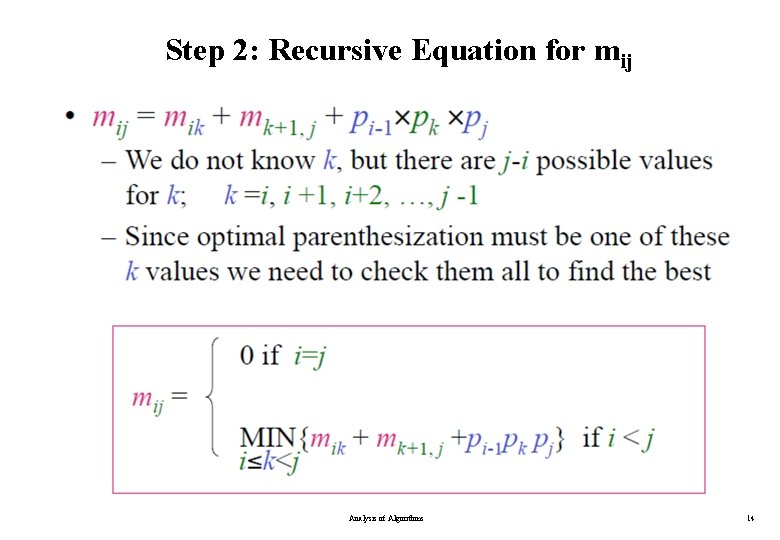
Step 2: Recursive Equation for mij Analysis of Algorithms 14

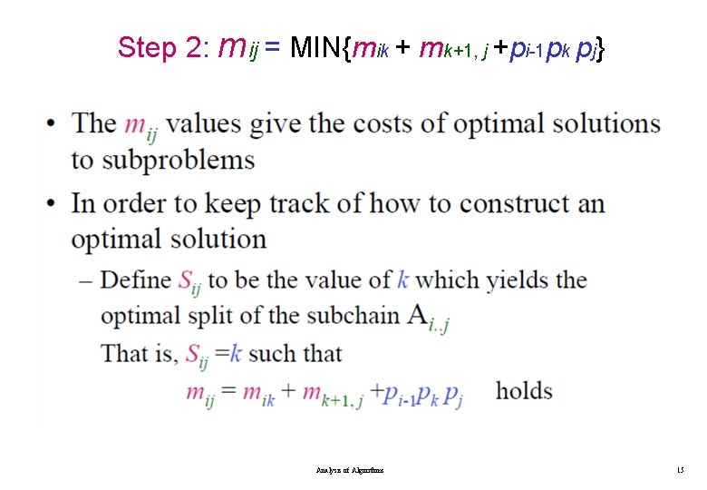
Step 2: mij = MIN{mik + mk+1, j +pi-1 pk pj} Analysis of Algorithms 15

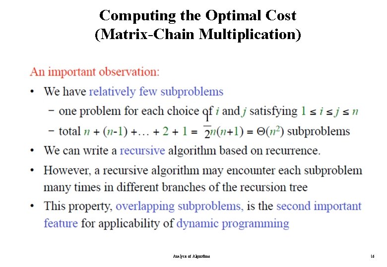
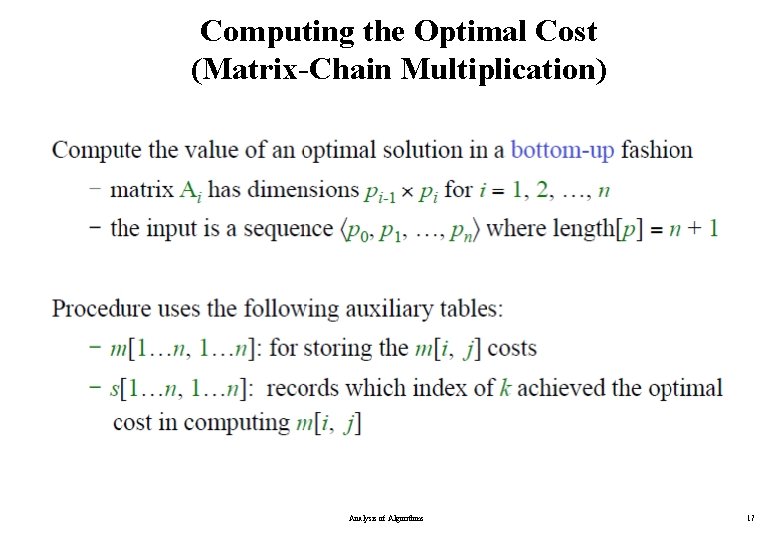
Computing the Optimal Cost (Matrix-Chain Multiplication) Analysis of Algorithms 16

Computing the Optimal Cost (Matrix-Chain Multiplication) Analysis of Algorithms 17

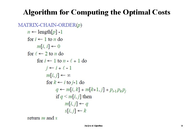
Algorithm for Computing the Optimal Costs Analysis of Algorithms 18

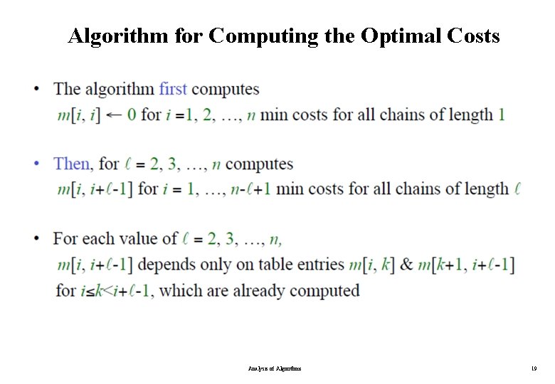
Algorithm for Computing the Optimal Costs Analysis of Algorithms 19

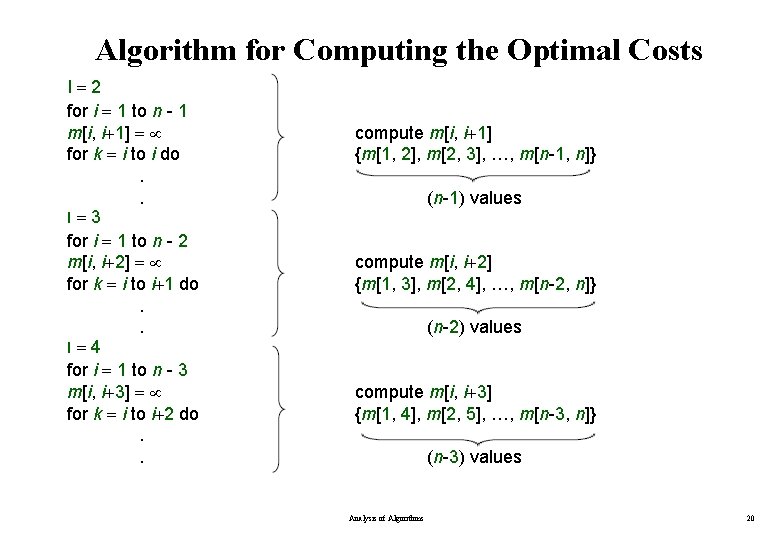
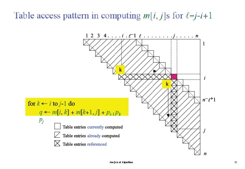
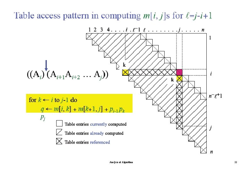
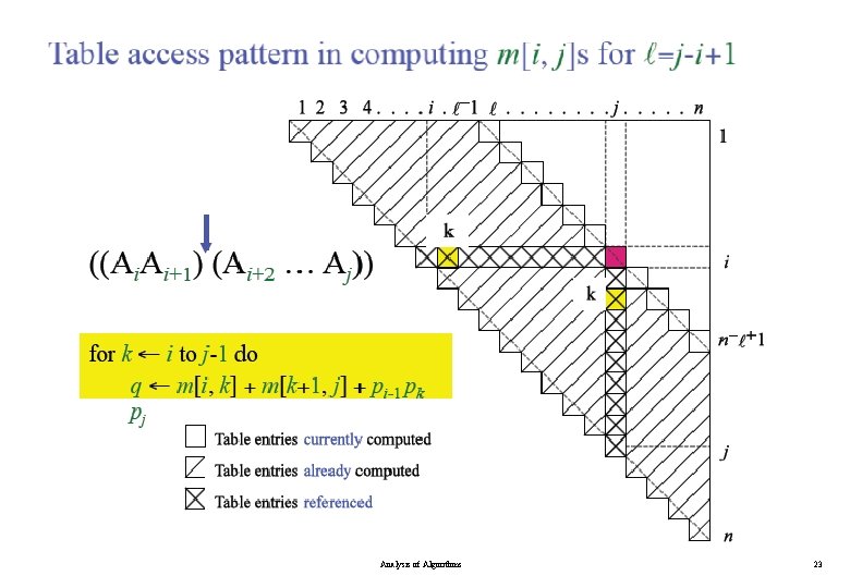
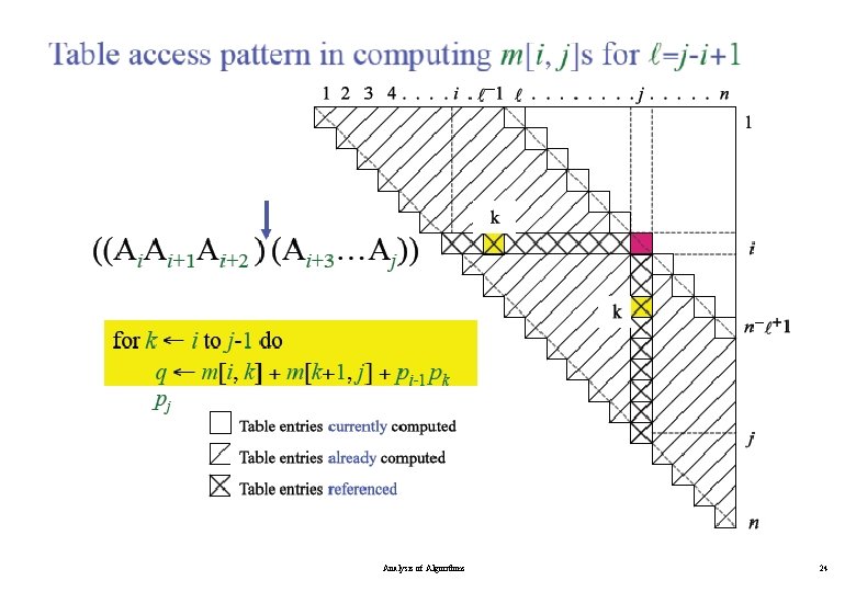
Algorithm for Computing the Optimal Costs l=2 for i = 1 to n - 1 m[i, i+1] = for k = i to i do. . l=3 for i = 1 to n - 2 m[i, i+2] = for k = i to i+1 do. . l=4 for i = 1 to n - 3 m[i, i+3] = for k = i to i+2 do. . compute m[i, i+1] {m[1, 2], m[2, 3], …, m[n-1, n]} (n-1) values compute m[i, i+2] {m[1, 3], m[2, 4], …, m[n-2, n]} (n-2) values compute m[i, i+3] {m[1, 4], m[2, 5], …, m[n-3, n]} (n-3) values Analysis of Algorithms 20

Analysis of Algorithms 21

Analysis of Algorithms 22

Analysis of Algorithms 23

Analysis of Algorithms 24

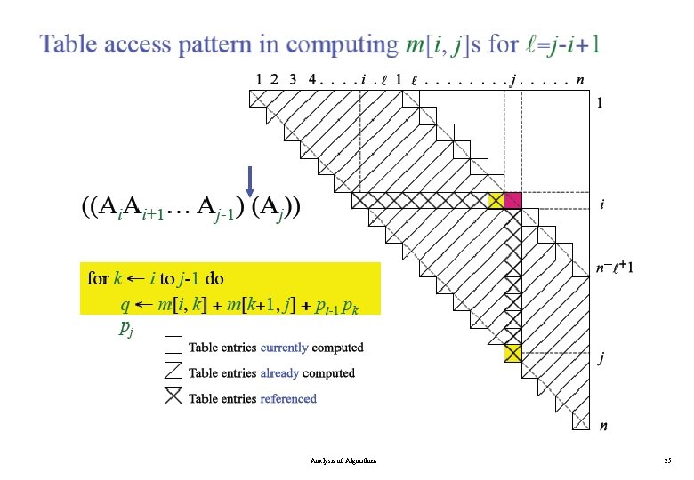
Analysis of Algorithms 25

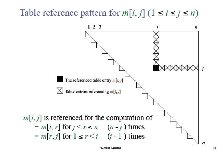
Analysis of Algorithms 26

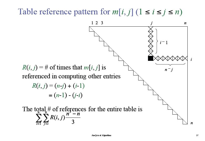
Analysis of Algorithms 27

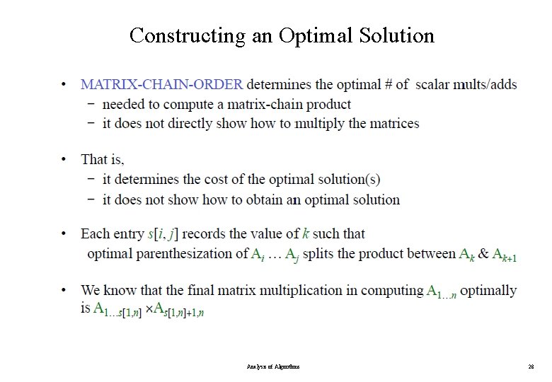
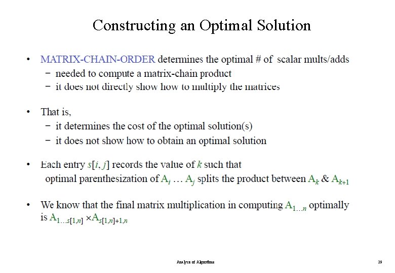
Constructing an Optimal Solution Analysis of Algorithms 28

Constructing an Optimal Solution Analysis of Algorithms 29

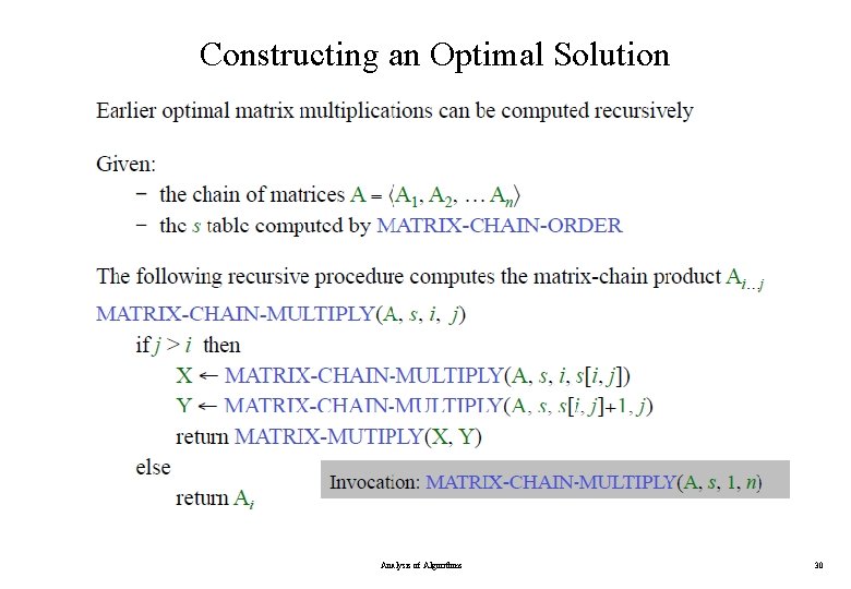
Constructing an Optimal Solution Analysis of Algorithms 30

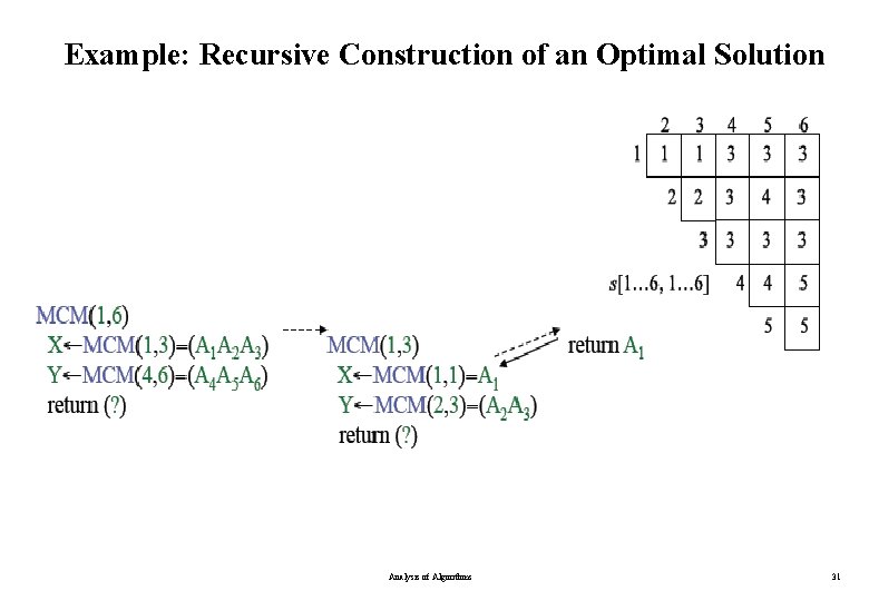
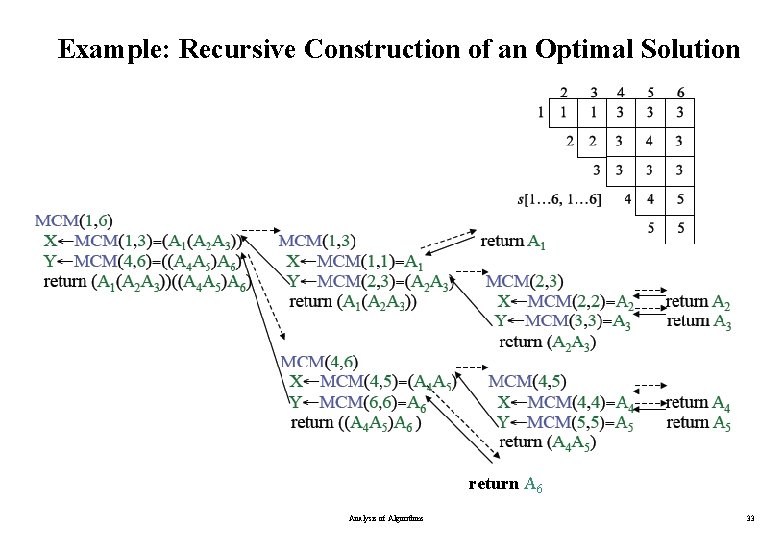
Example: Recursive Construction of an Optimal Solution Analysis of Algorithms 31

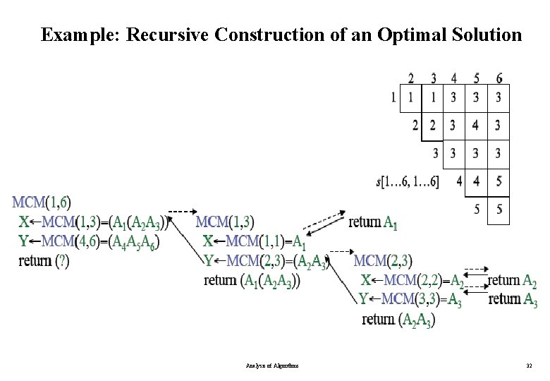
Example: Recursive Construction of an Optimal Solution Analysis of Algorithms 32

Example: Recursive Construction of an Optimal Solution return A 6 Analysis of Algorithms 33

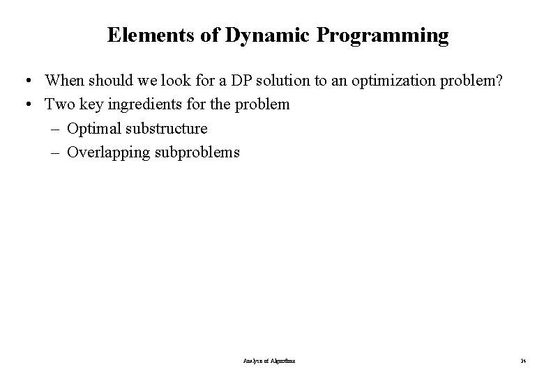
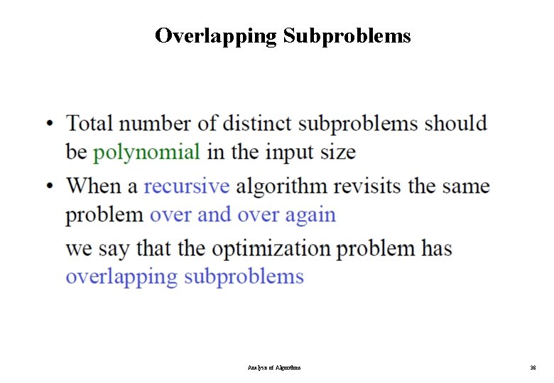
Elements of Dynamic Programming • When should we look for a DP solution to an optimization problem? • Two key ingredients for the problem – Optimal substructure – Overlapping subproblems Analysis of Algorithms 34

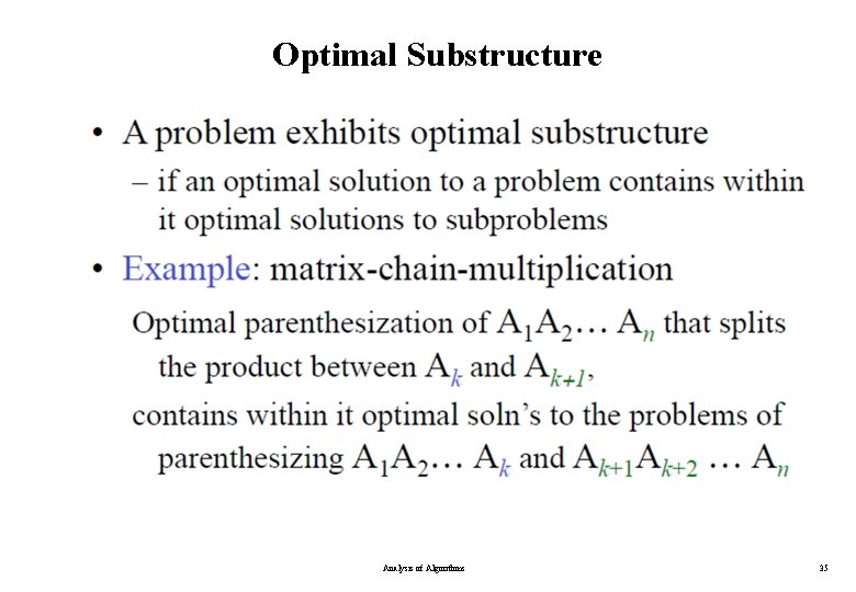
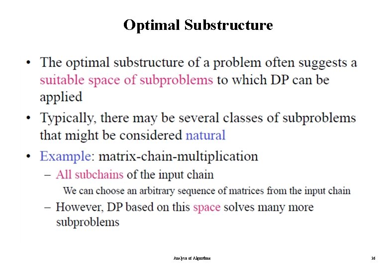
Optimal Substructure Analysis of Algorithms 35

Optimal Substructure Analysis of Algorithms 36

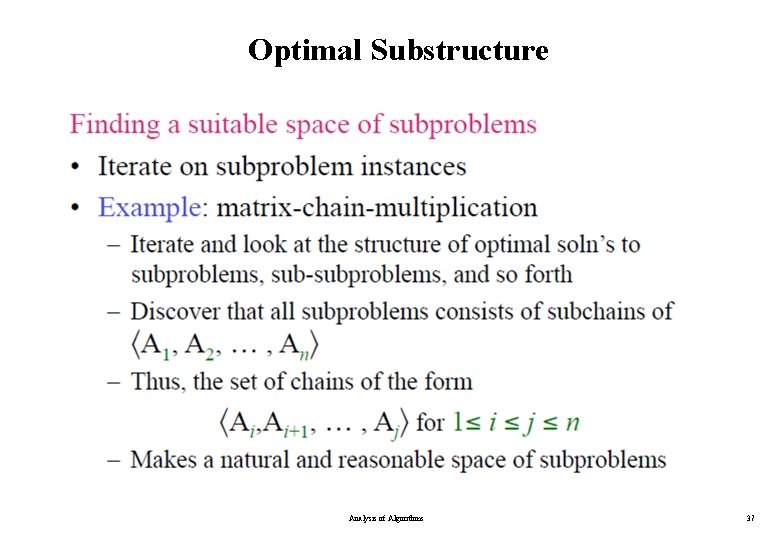
Optimal Substructure Analysis of Algorithms 37

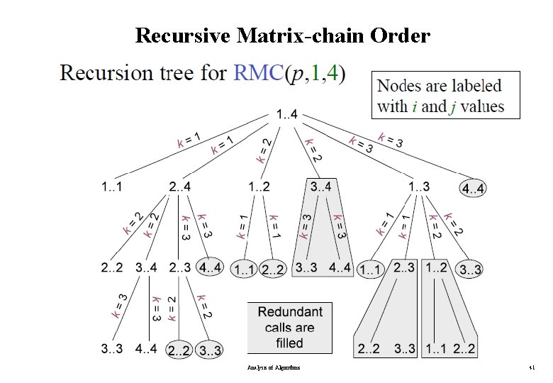
Overlapping Subproblems Analysis of Algorithms 38

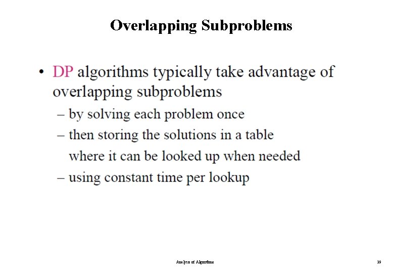
Overlapping Subproblems Analysis of Algorithms 39

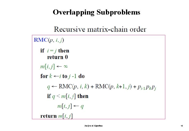
Overlapping Subproblems Analysis of Algorithms 40

Recursive Matrix-chain Order Analysis of Algorithms 41

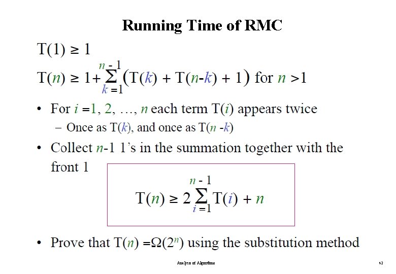
Running Time of RMC Analysis of Algorithms 42

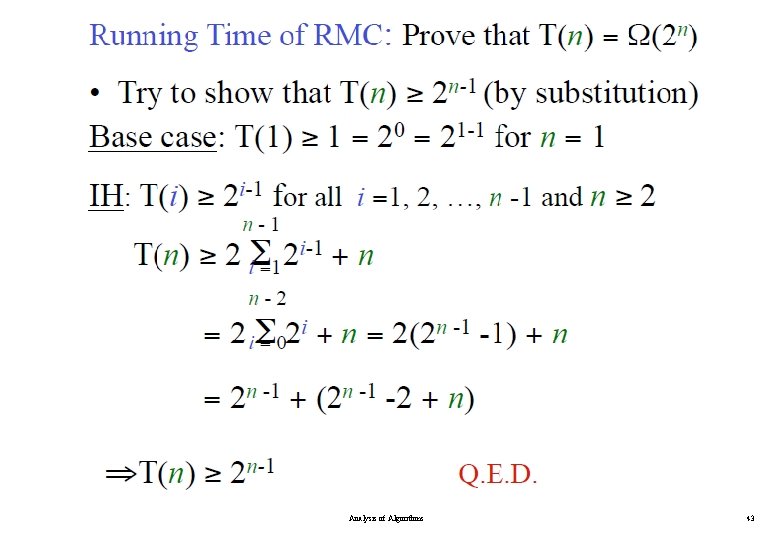
Analysis of Algorithms 43

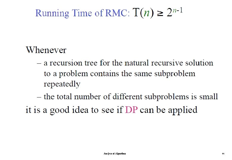
Analysis of Algorithms 44

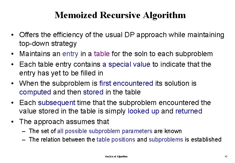
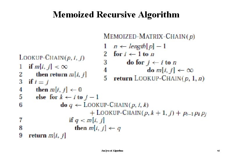
Memoized Recursive Algorithm • Offers the efficiency of the usual DP approach while maintaining top-down strategy • Maintains an entry in a table for the soln to each subproblem • Each table entry contains a special value to indicate that the entry has yet to be filled in • When the subproblem is first encountered its solution is computed and then stored in the table • Each subsequent time that the subproblem encountered the value stored in the table is simply looked up and returned • The approach assumes that – The set of all possible subproblem parameters are known – The relation between the table positions and subproblems is established Analysis of Algorithms 45

Memoized Recursive Algorithm Analysis of Algorithms 46

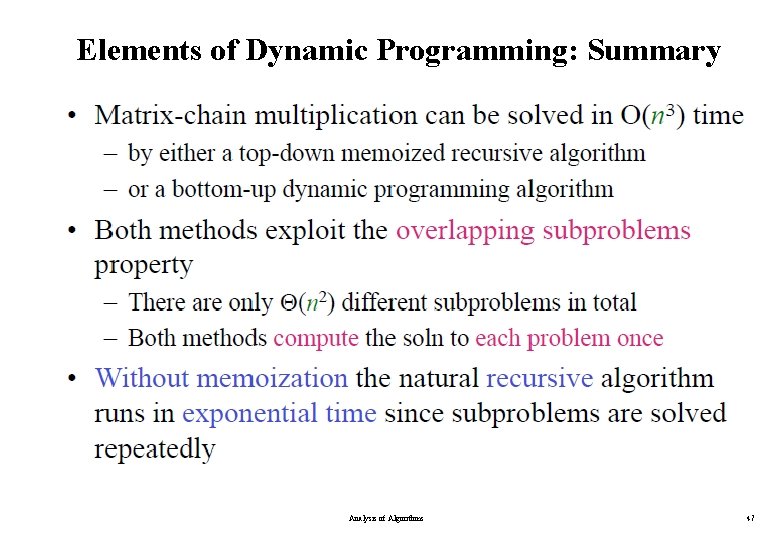
Elements of Dynamic Programming: Summary Analysis of Algorithms 47

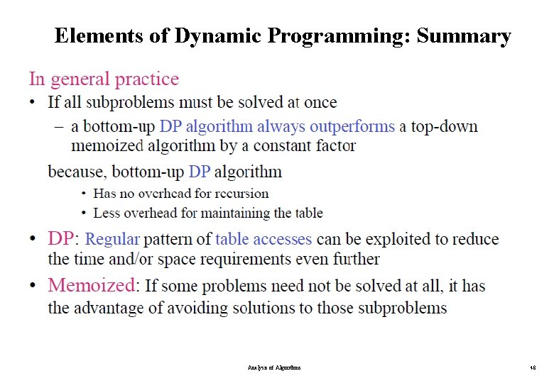
Elements of Dynamic Programming: Summary Analysis of Algorithms 48

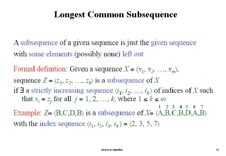
Longest Common Subsequence Analysis of Algorithms 49

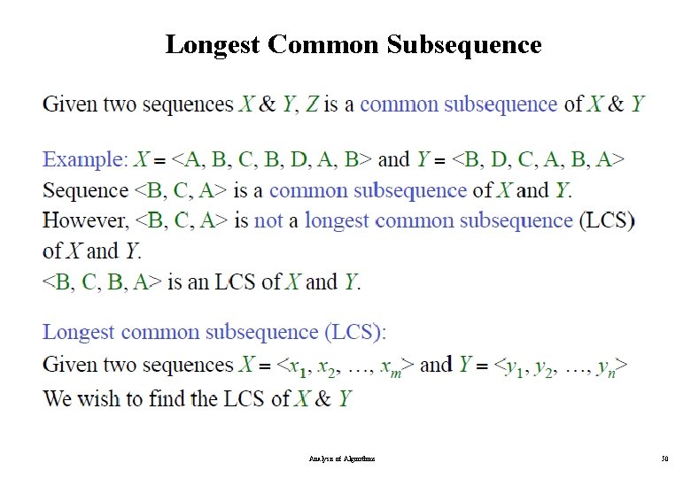
Longest Common Subsequence Analysis of Algorithms 50

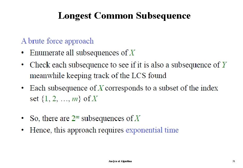
Longest Common Subsequence Analysis of Algorithms 51

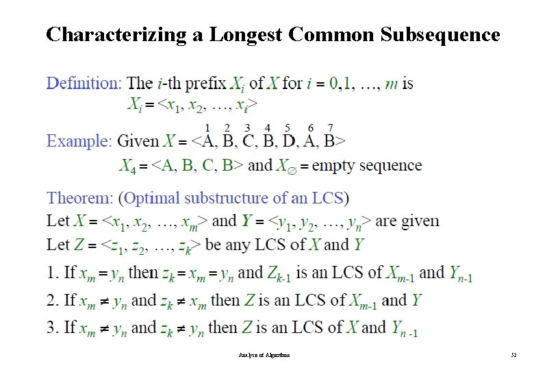
Characterizing a Longest Common Subsequence Analysis of Algorithms 52

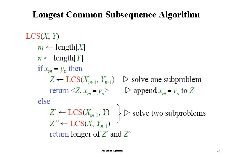
Longest Common Subsequence Algorithm Analysis of Algorithms 53

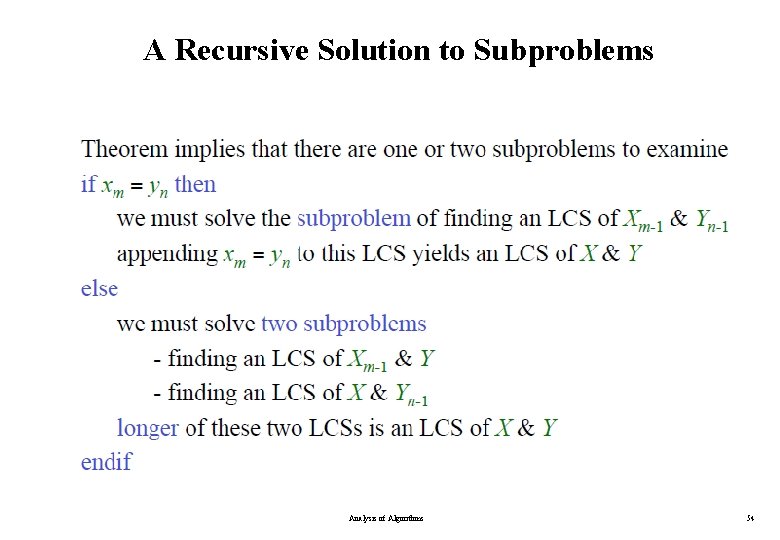
A Recursive Solution to Subproblems Analysis of Algorithms 54

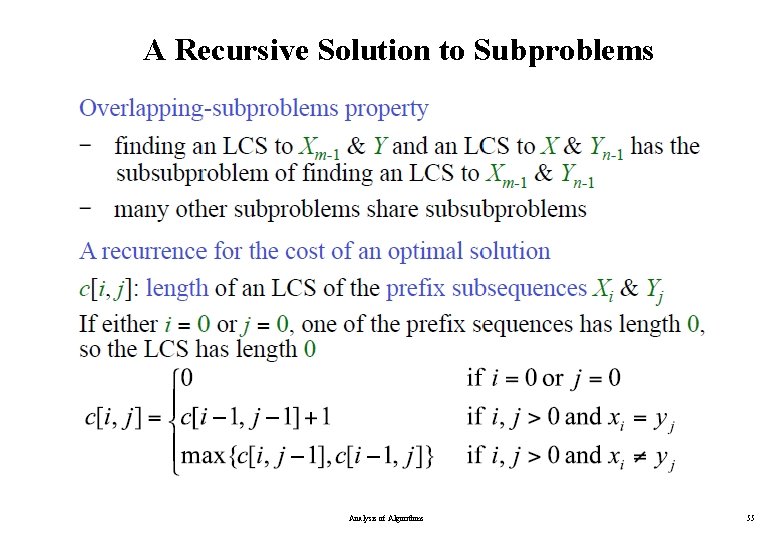
A Recursive Solution to Subproblems Analysis of Algorithms 55

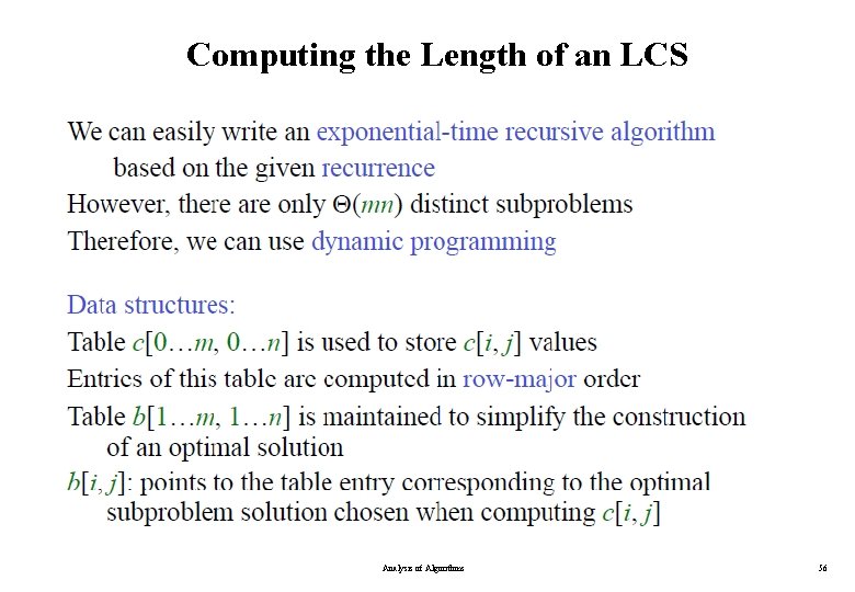
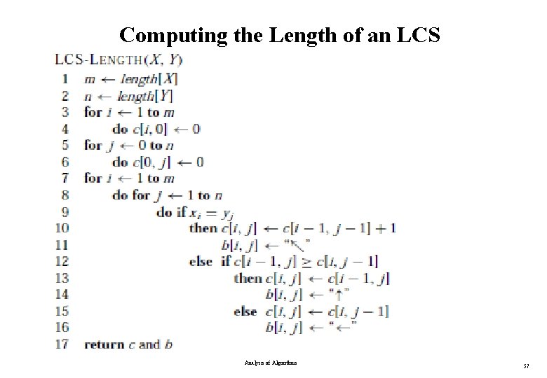
Computing the Length of an LCS Analysis of Algorithms 56

Computing the Length of an LCS Analysis of Algorithms 57

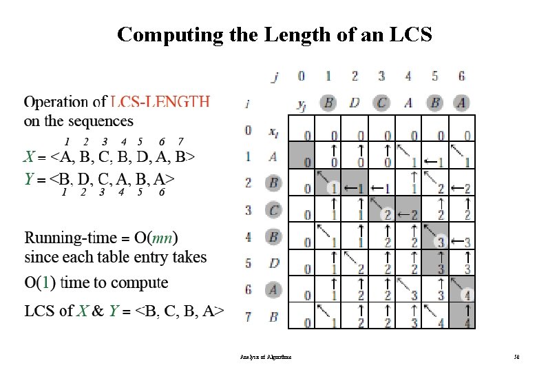
Computing the Length of an LCS Analysis of Algorithms 58

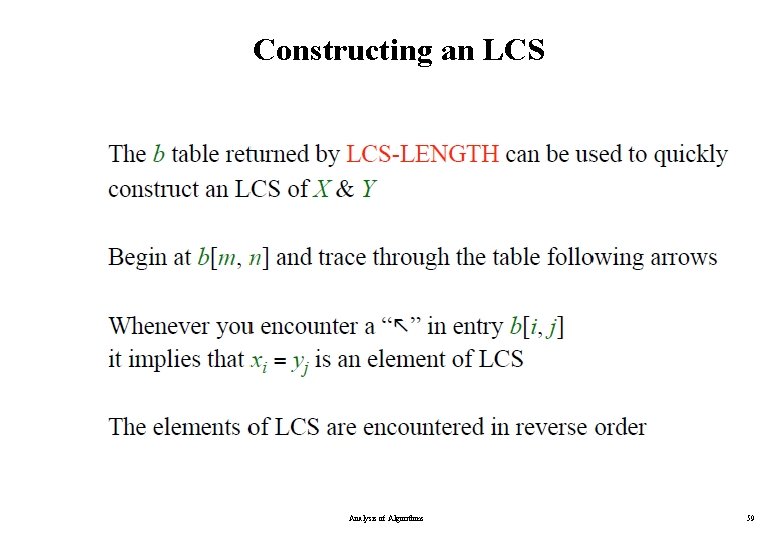
Constructing an LCS Analysis of Algorithms 59

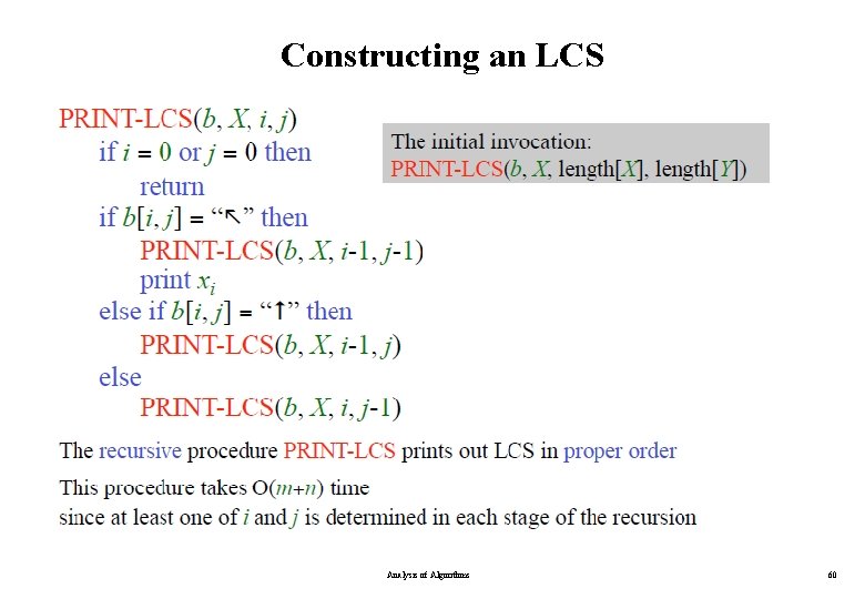
Constructing an LCS Analysis of Algorithms 60

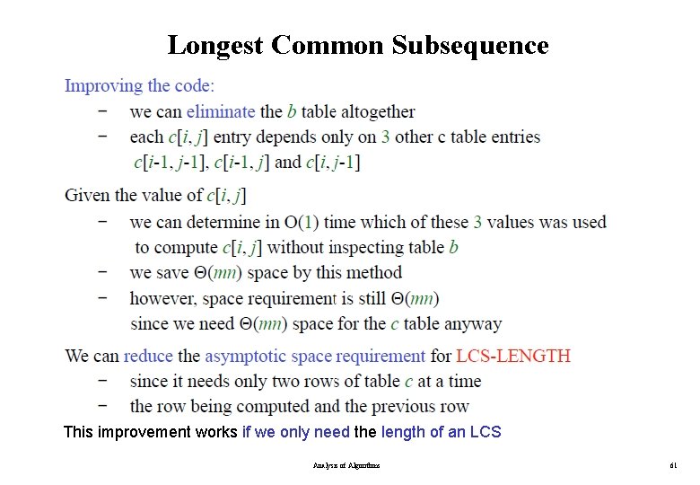
Longest Common Subsequence This improvement works if we only need the length of an LCS Analysis of Algorithms 61