Dynamic Programming Adapted from Introduction and Algorithms by

Dynamic Programming Adapted from Introduction and Algorithms by Kleinberg and Tardos.

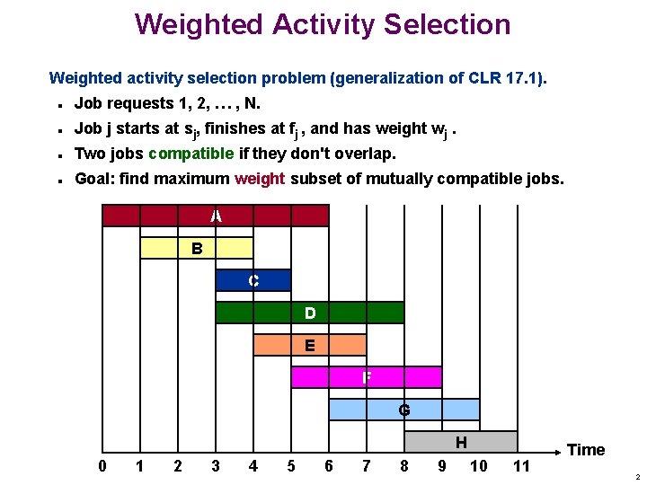
Weighted Activity Selection Weighted activity selection problem (generalization of CLR 17. 1). n n Job requests 1, 2, … , N. Job j starts at sj, finishes at fj , and has weight wj. n Two jobs compatible if they don't overlap. n Goal: find maximum weight subset of mutually compatible jobs. A B C D E F G H 0 1 2 3 4 5 6 7 8 9 10 11 Time 2

Activity Selection: Greedy Algorithm Recall greedy algorithm works if all weights are 1. Greedy Activity Selection Algorithm Sort jobs by increasing finish times so that f 1 f 2 . . . f. N. S = jobs selected. S = FOR j = 1 to N IF (job j compatible with A) S S {j} RETURN S 3

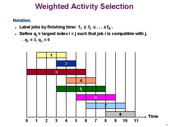
Weighted Activity Selection Notation. n n Label jobs by finishing time: f 1 f 2 . . . f. N. Define qj = largest index i < j such that job i is compatible with j. – q 7 = 3, q 2 = 0 1 2 3 4 5 6 7 8 9 10 11 Time 4

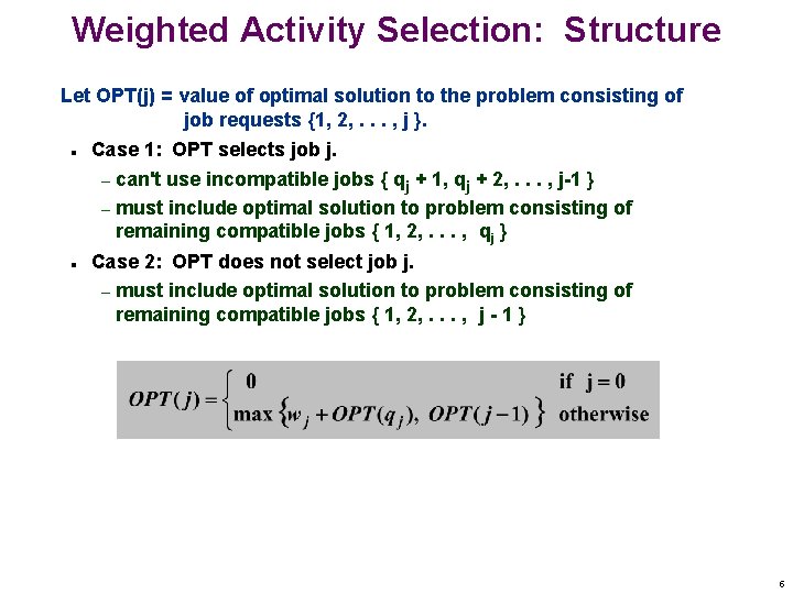
Weighted Activity Selection: Structure Let OPT(j) = value of optimal solution to the problem consisting of job requests {1, 2, . . . , j }. n n Case 1: OPT selects job j. – can't use incompatible jobs { qj + 1, qj + 2, . . . , j-1 } – must include optimal solution to problem consisting of remaining compatible jobs { 1, 2, . . . , qj } Case 2: OPT does not select job j. – must include optimal solution to problem consisting of remaining compatible jobs { 1, 2, . . . , j - 1 } 5

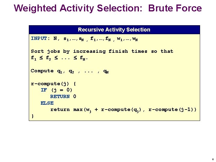
Weighted Activity Selection: Brute Force Recursive Activity Selection INPUT: N, s 1, …, s. N , f 1, …, f. N , w 1, …, w. N Sort jobs by increasing finish times so that f 1 f 2 . . . f. N. Compute q 1, q 2 , . . . , q. N r-compute(j) { IF (j = 0) RETURN 0 ELSE return max(wj + r-compute(qj), r-compute(j-1)) } 6

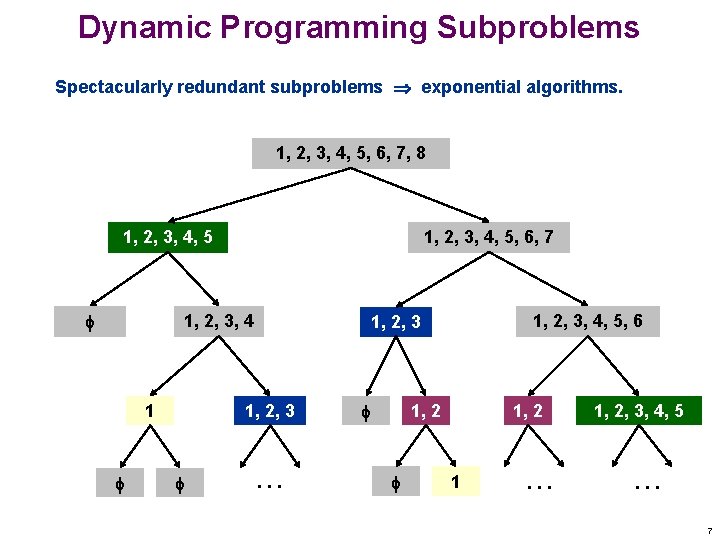
Dynamic Programming Subproblems Spectacularly redundant subproblems exponential algorithms. 1, 2, 3, 4, 5, 6, 7, 8 1, 2, 3, 4, 5, 6, 7 1, 2, 3, 4 1 1, 2, 3, 4, 5, 6 1, 2, 3 . . . 1, 2 1 . . . 1, 2, 3, 4, 5 . . . 7

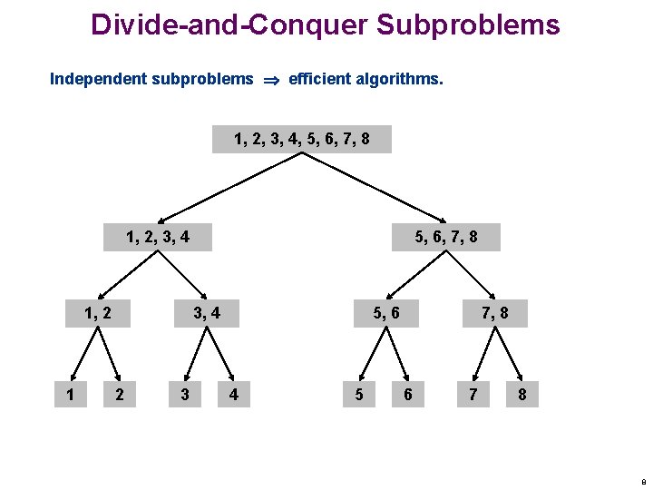
Divide-and-Conquer Subproblems Independent subproblems efficient algorithms. 1, 2, 3, 4, 5, 6, 7, 8 1, 2, 3, 4 1, 2 1 5, 6, 7, 8 3, 4 2 3 5, 6 4 5 7, 8 6 7 8 8

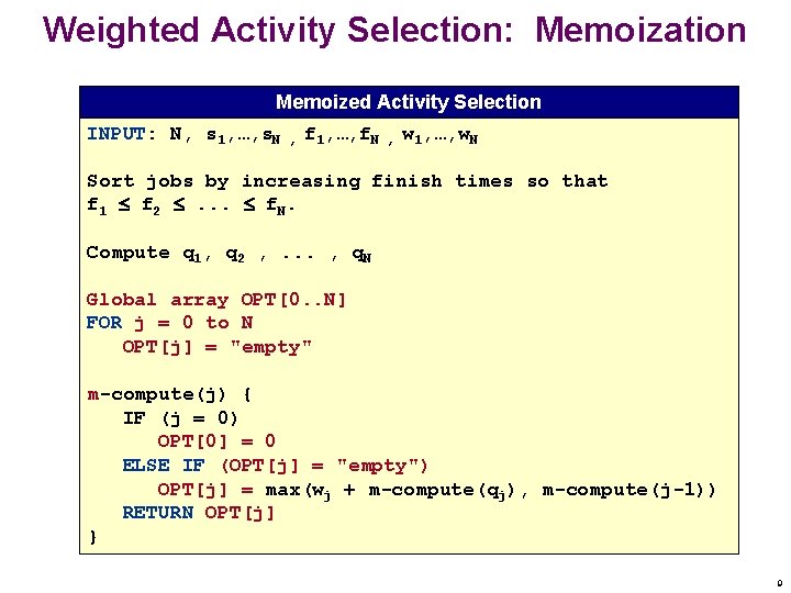
Weighted Activity Selection: Memoization Memoized Activity Selection INPUT: N, s 1, …, s. N , f 1, …, f. N , w 1, …, w. N Sort jobs by increasing finish times so that f 1 f 2 . . . f. N. Compute q 1, q 2 , . . . , q. N Global array OPT[0. . N] FOR j = 0 to N OPT[j] = "empty" m-compute(j) { IF (j = 0) OPT[0] = 0 ELSE IF (OPT[j] = "empty") OPT[j] = max(wj + m-compute(qj), m-compute(j-1)) RETURN OPT[j] } 9

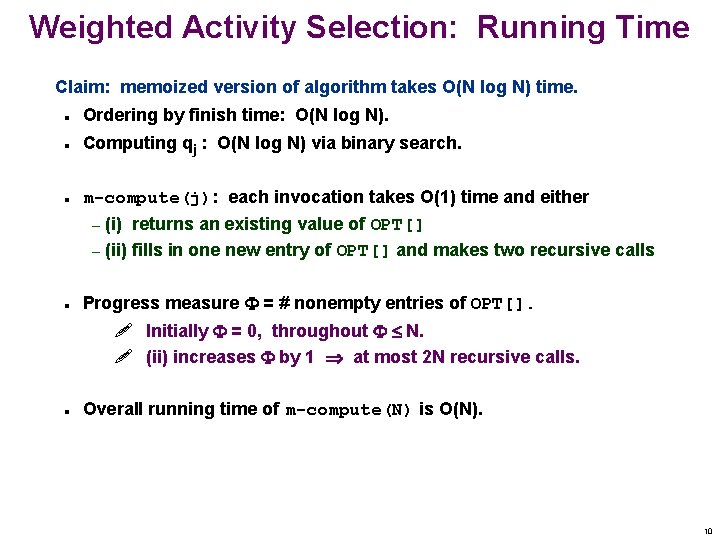
Weighted Activity Selection: Running Time Claim: memoized version of algorithm takes O(N log N) time. n n Ordering by finish time: O(N log N). Computing qj : O(N log N) via binary search. m-compute(j): each invocation takes O(1) time and either – (i) returns an existing value of OPT[] – (ii) fills in one new entry of OPT[] and makes two recursive calls Progress measure = # nonempty entries of OPT[]. ! Initially = 0, throughout N. ! (ii) increases by 1 at most 2 N recursive calls. n Overall running time of m-compute(N) is O(N). 10

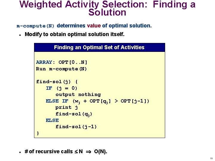
Weighted Activity Selection: Finding a Solution m-compute(N) determines value of optimal solution. n Modify to obtain optimal solution itself. Finding an Optimal Set of Activities ARRAY: OPT[0. . N] Run m-compute(N) find-sol(j) { IF (j = 0) output nothing ELSE IF (wj + OPT[qj] > OPT[j-1]) print j find-sol(qj) ELSE find-sol(j-1) } n # of recursive calls N O(N). 11

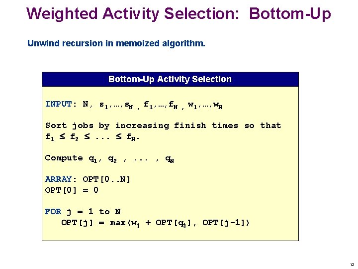
Weighted Activity Selection: Bottom-Up Unwind recursion in memoized algorithm. Bottom-Up Activity Selection INPUT: N, s 1, …, s. N , f 1, …, f. N , w 1, …, w. N Sort jobs by increasing finish times so that f 1 f 2 . . . f. N. Compute q 1, q 2 , . . . , q. N ARRAY: OPT[0. . N] OPT[0] = 0 FOR j = 1 to N OPT[j] = max(wj + OPT[qj], OPT[j-1]) 12

Dynamic Programming Overview Dynamic programming. n n Similar to divide-and-conquer. – solves problem by combining solution to sub-problems Different from divide-and-conquer. – sub-problems are not independent – save solutions to repeated sub-problems in table – solution usually has a natural left-to-right ordering Recipe. n Characterize structure of problem. – optimal substructure property n Recursively define value of optimal solution. n Compute value of optimal solution. n Construct optimal solution from computed information. Top-down vs. bottom-up: different people have different intuitions. 13

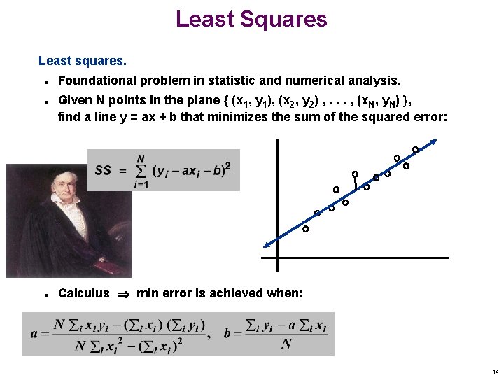
Least Squares Least squares. n n n Foundational problem in statistic and numerical analysis. Given N points in the plane { (x 1, y 1), (x 2, y 2) , . . . , (x. N, y. N) }, find a line y = ax + b that minimizes the sum of the squared error: Calculus min error is achieved when: 14

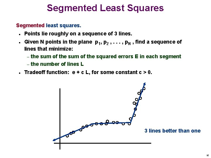
Segmented Least Squares Segmented least squares. n n n Points lie roughly on a sequence of 3 lines. Given N points in the plane p 1, p 2 , . . . , p. N , find a sequence of lines that minimize: – the sum of the squared errors E in each segment – the number of lines L Tradeoff function: e + c L, for some constant c > 0. 3 lines better than one 15

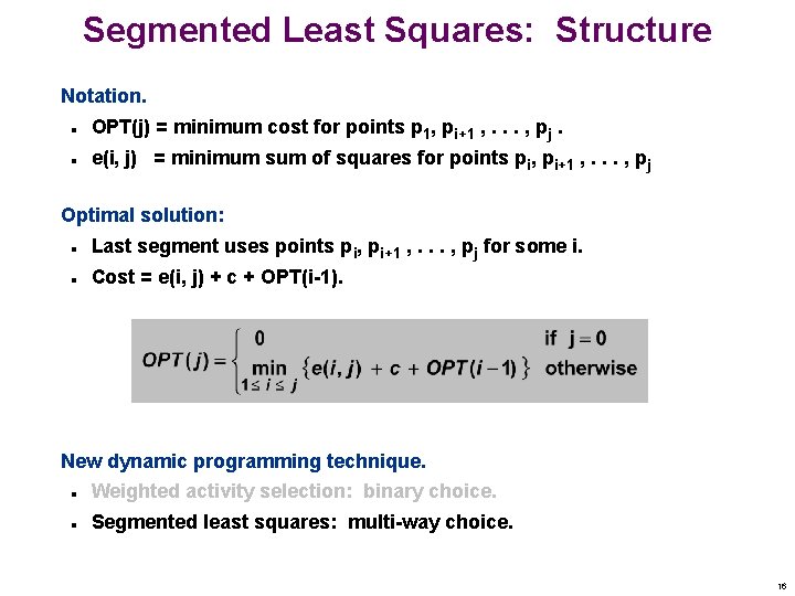
Segmented Least Squares: Structure Notation. n OPT(j) = minimum cost for points p 1, pi+1 , . . . , pj. n e(i, j) = minimum sum of squares for points pi, pi+1 , . . . , pj Optimal solution: n n Last segment uses points pi, pi+1 , . . . , pj for some i. Cost = e(i, j) + c + OPT(i-1). New dynamic programming technique. n Weighted activity selection: binary choice. n Segmented least squares: multi-way choice. 16

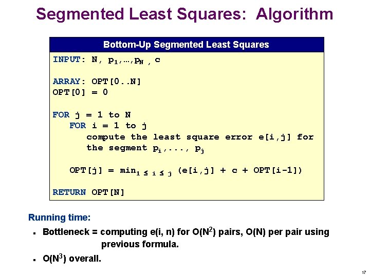
Segmented Least Squares: Algorithm Bottom-Up Segmented Least Squares INPUT: N, p 1, …, p. N , c ARRAY: OPT[0. . N] OPT[0] = 0 FOR j = 1 to N FOR i = 1 to j compute the least square error e[i, j] for the segment pi, . . . , pj OPT[j] = min 1 i j (e[i, j] + c + OPT[i-1]) RETURN OPT[N] Running time: n n Bottleneck = computing e(i, n) for O(N 2) pairs, O(N) per pair using previous formula. O(N 3) overall. 17

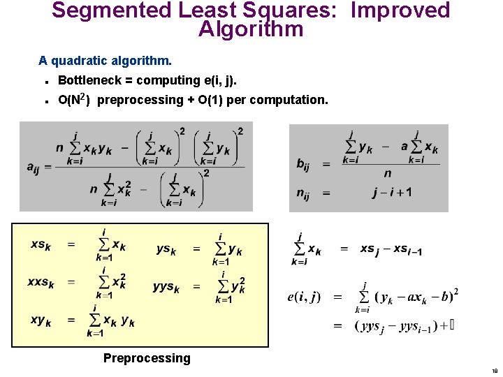
Segmented Least Squares: Improved Algorithm A quadratic algorithm. n Bottleneck = computing e(i, j). n O(N 2) preprocessing + O(1) per computation. Preprocessing 18

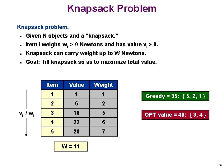
Knapsack Problem Knapsack problem. n n Given N objects and a "knapsack. " Item i weighs wi > 0 Newtons and has value vi > 0. n Knapsack can carry weight up to W Newtons. n Goal: fill knapsack so as to maximize total value. vi / w i Item Value Weight 1 1 1 2 6 2 3 18 5 4 22 6 5 28 7 Greedy = 35: { 5, 2, 1 } OPT value = 40: { 3, 4 } W = 11 19

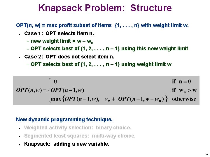
Knapsack Problem: Structure OPT(n, w) = max profit subset of items {1, . . . , n} with weight limit w. n n Case 1: OPT selects item n. – new weight limit = w – wn – OPT selects best of {1, 2, . . . , n – 1} using this new weight limit Case 2: OPT does not select item n. – OPT selects best of {1, 2, . . . , n – 1} using weight limit w New dynamic programming technique. n Weighted activity selection: binary choice. n Segmented least squares: multi-way choice. n Knapsack: adding a new variable. 20

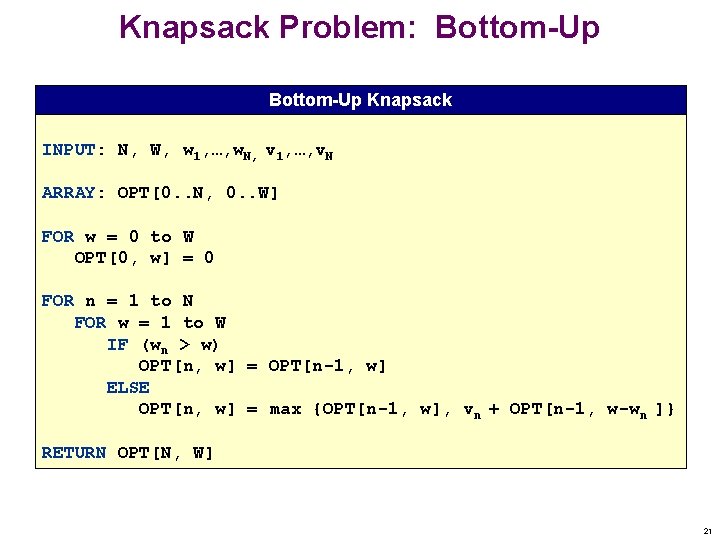
Knapsack Problem: Bottom-Up Knapsack INPUT: N, W, w 1, …, w. N, v 1, …, v. N ARRAY: OPT[0. . N, 0. . W] FOR w = 0 to W OPT[0, w] = 0 FOR n = 1 to N FOR w = 1 to W IF (wn > w) OPT[n, w] = OPT[n-1, w] ELSE OPT[n, w] = max {OPT[n-1, w], vn + OPT[n-1, w-wn ]} RETURN OPT[N, W] 21

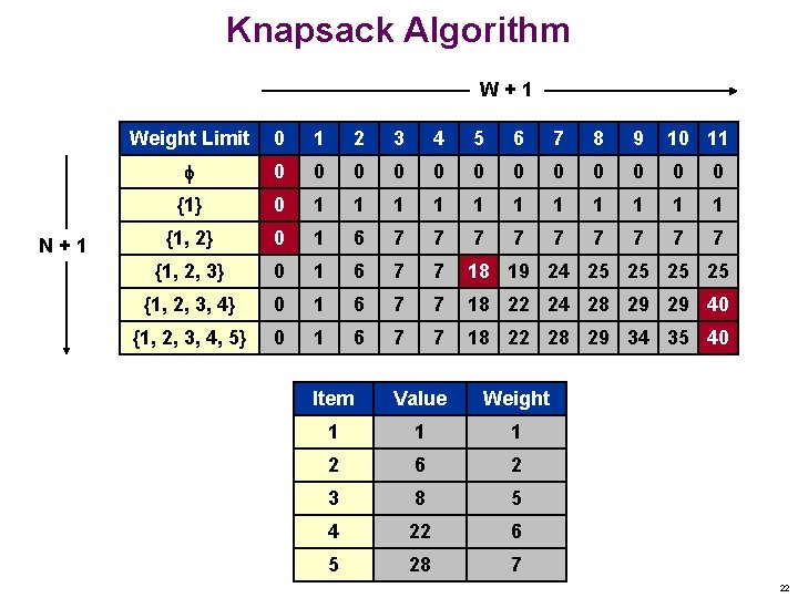
Knapsack Algorithm W+1 N+1 Weight Limit 0 1 2 3 4 5 6 7 8 9 10 11 0 0 0 {1} 0 1 1 1 {1, 2} 0 1 6 7 7 7 7 7 {1, 2, 3} 0 1 6 7 7 18 19 24 25 25 {1, 2, 3, 4} 0 1 6 7 7 18 22 24 28 29 29 40 {1, 2, 3, 4, 5} 0 1 6 7 7 18 22 28 29 34 35 40 Item Value Weight 1 1 1 2 6 2 3 8 5 4 22 6 5 28 7 22

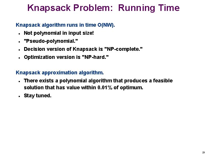
Knapsack Problem: Running Time Knapsack algorithm runs in time O(NW). n Not polynomial in input size! n "Pseudo-polynomial. " n Decision version of Knapsack is "NP-complete. " n Optimization version is "NP-hard. " Knapsack approximation algorithm. n n There exists a polynomial algorithm that produces a feasible solution that has value within 0. 01% of optimum. Stay tuned. 23

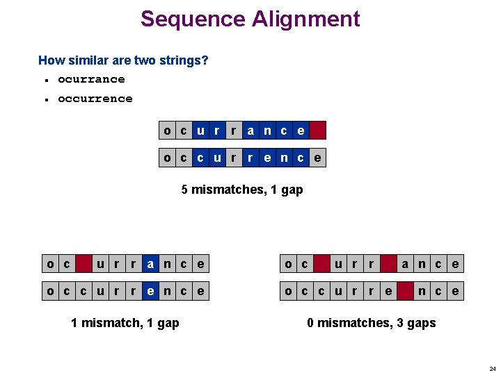
Sequence Alignment How similar are two strings? ocurrance n n occurrence o c u r r a n c e o c c u r r e n c e 5 mismatches, 1 gap o c u r r a n c e o c c u r r e n c e 1 mismatch, 1 gap o c u r r o c c u r r e a n c e 0 mismatches, 3 gaps 24

Industrial Application 25

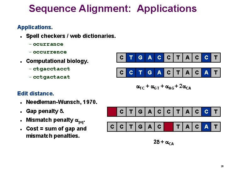
Sequence Alignment: Applications. n n Spell checkers / web dictionaries. – ocurrance – occurrence Computational biology. – ctgacct – cctgactacat C T G A C T A C C T T A C A T TC + GT + AG+ 2 CA Edit distance. n Needleman-Wunsch, 1970. n Gap penalty . n n Mismatch penalty pq. Cost = sum of gap and mismatch penalties. C C C T G A C C T T G A C T A C A T 2 + CA 26

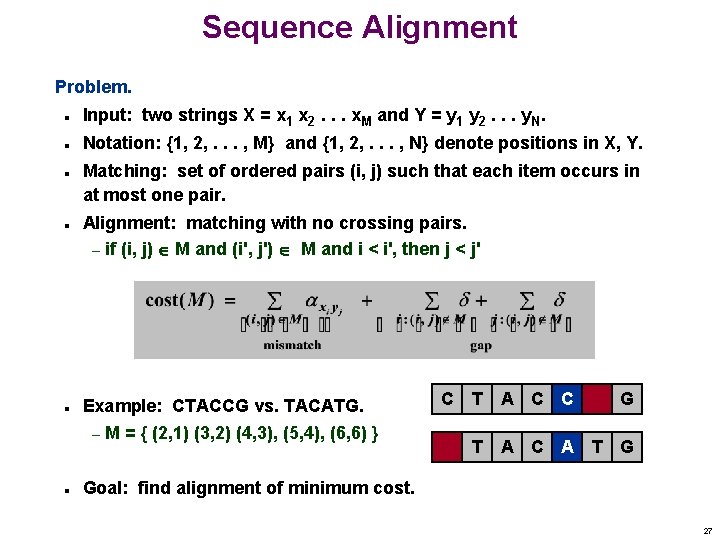
Sequence Alignment Problem. n n n Input: two strings X = x 1 x 2. . . x. M and Y = y 1 y 2. . . y. N. Notation: {1, 2, . . . , M} and {1, 2, . . . , N} denote positions in X, Y. Matching: set of ordered pairs (i, j) such that each item occurs in at most one pair. Alignment: matching with no crossing pairs. – if (i, j) M and (i', j') M and i < i', then j < j' Example: CTACCG vs. TACATG. – M = { (2, 1) (3, 2) (4, 3), (5, 4), (6, 6) } C T A C C G T A C A T G Goal: find alignment of minimum cost. 27

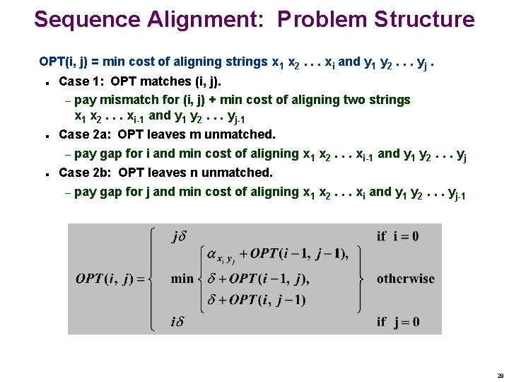
Sequence Alignment: Problem Structure OPT(i, j) = min cost of aligning strings x 1 x 2. . . xi and y 1 y 2. . . yj. n n n Case 1: OPT matches (i, j). – pay mismatch for (i, j) + min cost of aligning two strings x 1 x 2. . . xi-1 and y 1 y 2. . . yj-1 Case 2 a: OPT leaves m unmatched. – pay gap for i and min cost of aligning x 1 x 2. . . xi-1 and y 1 y 2. . . yj Case 2 b: OPT leaves n unmatched. – pay gap for j and min cost of aligning x 1 x 2. . . xi and y 1 y 2. . . yj-1 28

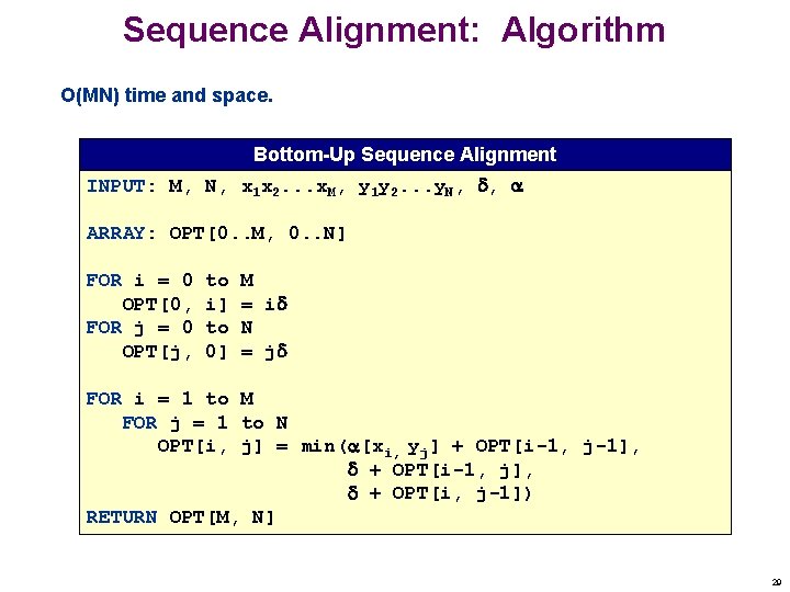
Sequence Alignment: Algorithm O(MN) time and space. Bottom-Up Sequence Alignment INPUT: M, N, x 1 x 2. . . x. M, y 1 y 2. . . y. N, , ARRAY: OPT[0. . M, 0. . N] FOR i = 0 OPT[0, FOR j = 0 OPT[j, to i] to 0] M = i N = j FOR i = 1 to M FOR j = 1 to N OPT[i, j] = min( [xi, yj] + OPT[i-1, j-1], + OPT[i-1, j], + OPT[i, j-1]) RETURN OPT[M, N] 29

Sequence Alignment: Linear Space Straightforward dynamic programming takes (MN) time and space. n n English words or sentences may not be a problem. Computational biology huge problem. – M = N = 100, 000 – 10 billion ops OK, but 10 gigabyte array? Optimal value in O(M + N) space and O(MN) time. n Only need to remember OPT( i - 1, • ) to compute OPT( i, • ). n Not clear how to recover optimal alignment itself. Optimal alignment in O(M + N) space and O(MN) time. n Clever combination of divide-and-conquer and dynamic programming. 30

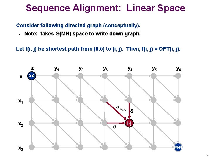
Sequence Alignment: Linear Space Consider following directed graph (conceptually). n Note: takes (MN) space to write down graph. Let f(i, j) be shortest path from (0, 0) to (i, j). Then, f(i, j) = OPT(i, j). y 1 y 2 y 3 y 4 y 5 y 6 0 -0 x 1 x 2 x 3 i-j M-N 31

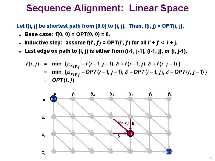
Sequence Alignment: Linear Space Let f(i, j) be shortest path from (0, 0) to (i, j). Then, f(i, j) = OPT(i, j). n Base case: f(0, 0) = OPT(0, 0) = 0. n Inductive step: assume f(i', j') = OPT(i', j') for all i' + j' < i + j. n Last edge on path to (i, j) is either from (i-1, j-1), (i-1, j), or (i, j-1). y 1 y 2 y 3 y 4 y 5 y 6 0 -0 x 1 x 2 x 3 i-j M-N 32

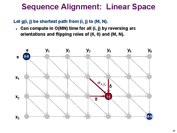
Sequence Alignment: Linear Space Let g(i, j) be shortest path from (i, j) to (M, N). n Can compute in O(MN) time for all (i, j) by reversing arc orientations and flipping roles of (0, 0) and (M, N). y 1 y 2 y 3 y 4 y 5 y 6 0 -0 x 1 x 2 x 3 i-j M-N 33

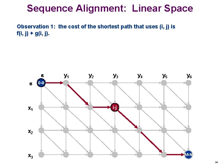
Sequence Alignment: Linear Space Observation 1: the cost of the shortest path that uses (i, j) is f(i, j) + g(i, j). x 1 y 2 y 3 y 4 y 5 y 6 0 -0 i-j x 2 x 3 M-N 34

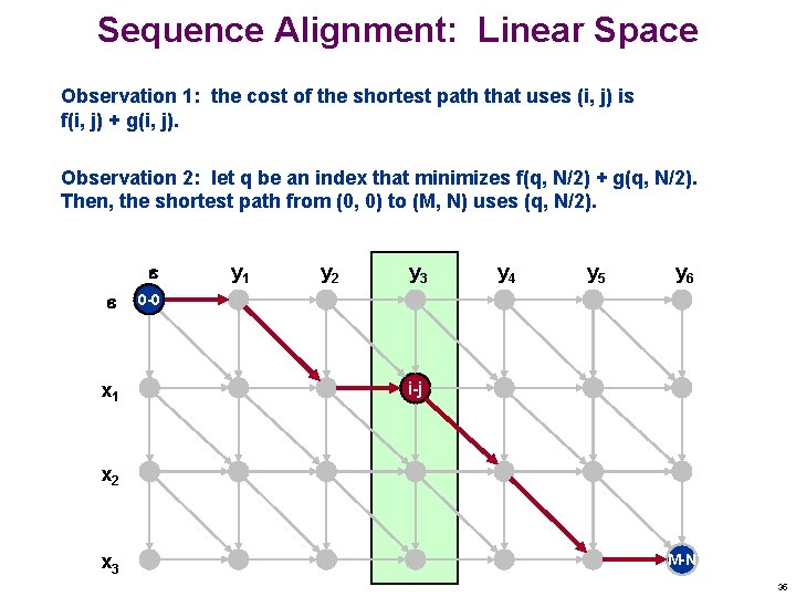
Sequence Alignment: Linear Space Observation 1: the cost of the shortest path that uses (i, j) is f(i, j) + g(i, j). Observation 2: let q be an index that minimizes f(q, N/2) + g(q, N/2). Then, the shortest path from (0, 0) to (M, N) uses (q, N/2). x 1 y 2 y 3 y 4 y 5 y 6 0 -0 i-j x 2 x 3 M-N 35

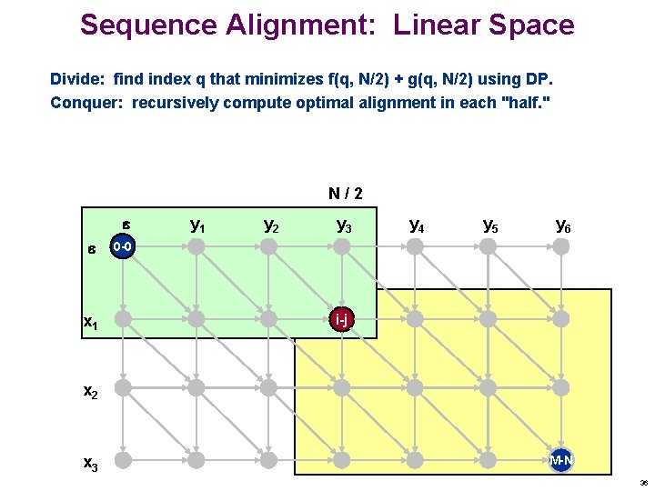
Sequence Alignment: Linear Space Divide: find index q that minimizes f(q, N/2) + g(q, N/2) using DP. Conquer: recursively compute optimal alignment in each "half. " N/2 x 1 y 2 y 3 y 4 y 5 y 6 0 -0 i-j x 2 x 3 M-N 36

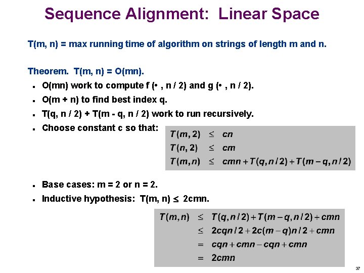
Sequence Alignment: Linear Space T(m, n) = max running time of algorithm on strings of length m and n. Theorem. T(m, n) = O(mn). n O(mn) work to compute f ( • , n / 2) and g ( • , n / 2). n O(m + n) to find best index q. n T(q, n / 2) + T(m - q, n / 2) work to run recursively. n Choose constant c so that: n Base cases: m = 2 or n = 2. n Inductive hypothesis: T(m, n) 2 cmn. 37