Dynamic Program Analysis Xiangyu Zhang Introduction Dynamic program

Dynamic Program Analysis Xiangyu Zhang

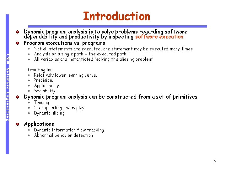
Introduction Dynamic program analysis is to solve problems regarding software dependability and productivity by inspecting software execution. Program executions vs. programs CS 510 Not all statements are executed; one statement may be executed many times. Analysis on a single path – the executed path All variables are instantiated (solving the aliasing problem) Software Engineering Resulting in: Relatively lower learning curve. Precision. Applicability. Scalability. Dynamic program analysis can be constructed from a set of primitives Tracing Checkpointing and replay Dynamic slicing Applications Dynamic information flow tracking Abnormal behavior detection 2

Program Tracing

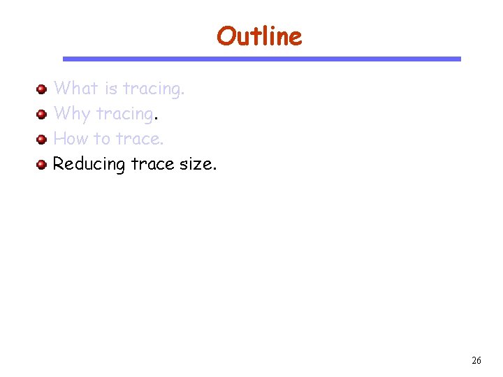
Outline CS 510 Software Engineering What is tracing. Why tracing. How to trace. Reducing trace size. 4

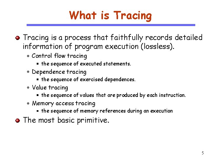
What is Tracing CS 510 Tracing is a process that faithfully records detailed information of program execution (lossless). Control flow tracing Software Engineering the sequence of executed statements. Dependence tracing the sequence of exercised dependences. Value tracing the sequence of values that are produced by each instruction. Memory access tracing the sequence of memory references during an execution The most basic primitive. 5

Why Tracing CS 510 Malware analysis Abnormal behavior detection Forensic analysis Software Engineering 6

Outline CS 510 Software Engineering What is tracing. Why tracing. How to trace. Reducing trace size. Trace accessibility 7

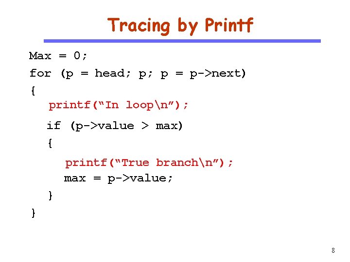
Tracing by Printf CS 510 Software Engineering Max = 0; for (p = head; p; p = p->next) { printf(“In loopn”); if (p->value > max) { printf(“True branchn”); max = p->value; } } 8

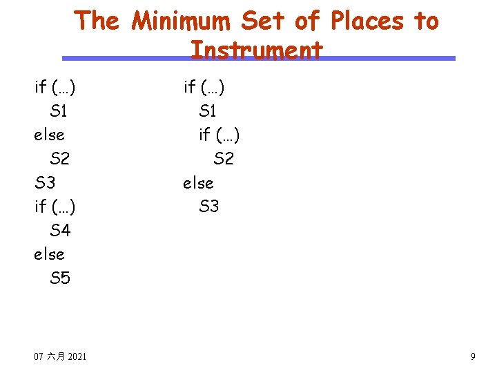
The Minimum Set of Places to Instrument CS 510 Software Engineering if (…) S 1 else S 2 S 3 if (…) S 4 else S 5 07 六月 2021 if (…) S 2 else S 3 9

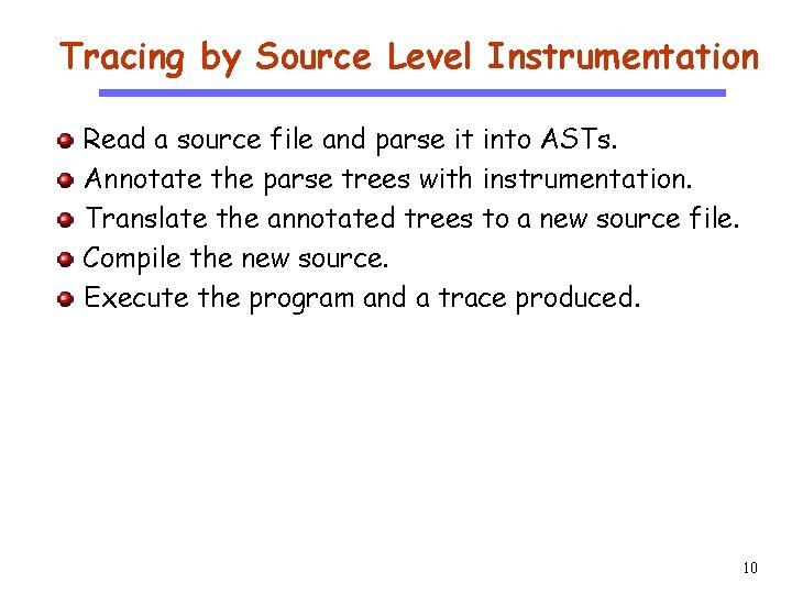
Tracing by Source Level Instrumentation CS 510 Software Engineering Read a source file and parse it into ASTs. Annotate the parse trees with instrumentation. Translate the annotated trees to a new source file. Compile the new source. Execute the program and a trace produced. 10

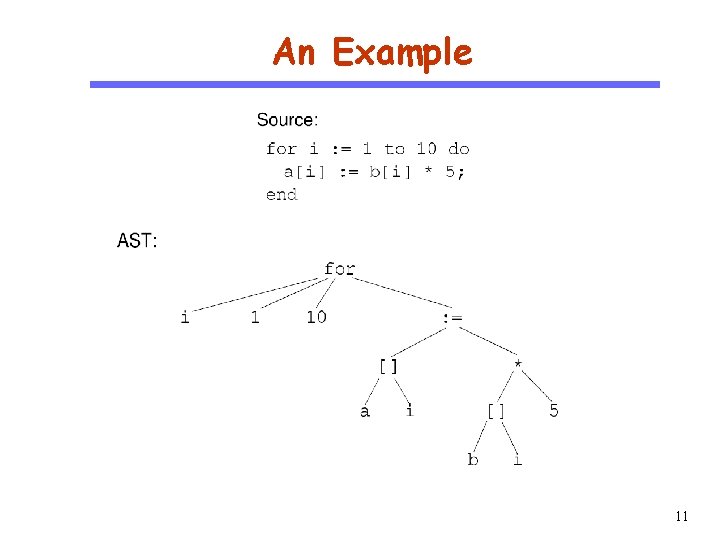
An Example CS 510 Software Engineering 11

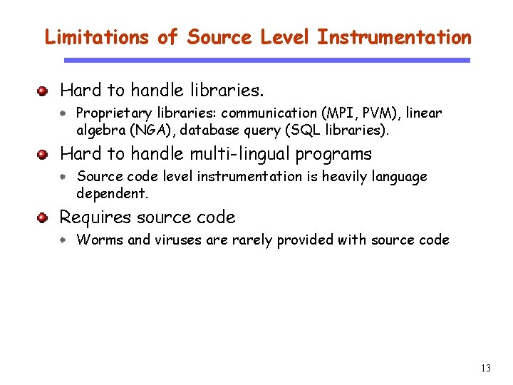
Limitations of Source Level Instrumentation Hard to handle libraries. CS 510 Proprietary libraries: communication (MPI, PVM), linear algebra (NGA), database query (SQL libraries). Software Engineering Hard to handle multi-lingual programs Source code level instrumentation is heavily language dependent. Requires source code Worms and viruses are rarely provided with source code 13

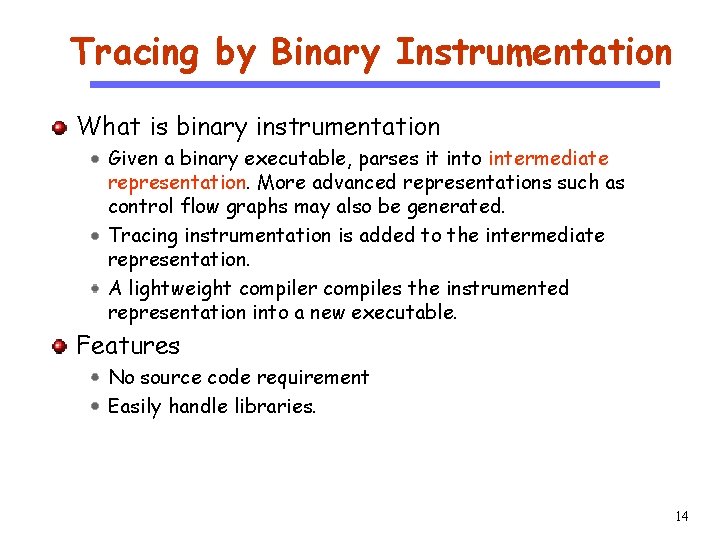
Tracing by Binary Instrumentation What is binary instrumentation CS 510 Software Engineering Given a binary executable, parses it into intermediate representation. More advanced representations such as control flow graphs may also be generated. Tracing instrumentation is added to the intermediate representation. A lightweight compiler compiles the instrumented representation into a new executable. Features No source code requirement Easily handle libraries. 14

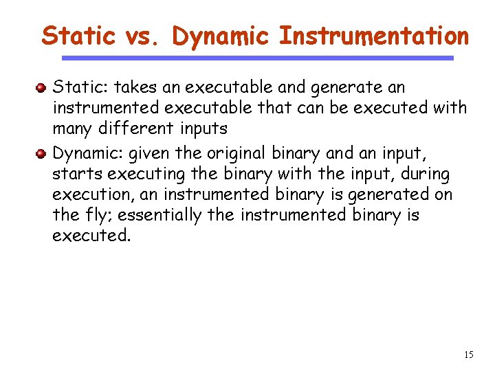
Static vs. Dynamic Instrumentation CS 510 Software Engineering Static: takes an executable and generate an instrumented executable that can be executed with many different inputs Dynamic: given the original binary and an input, starts executing the binary with the input, during execution, an instrumented binary is generated on the fly; essentially the instrumented binary is executed. 15

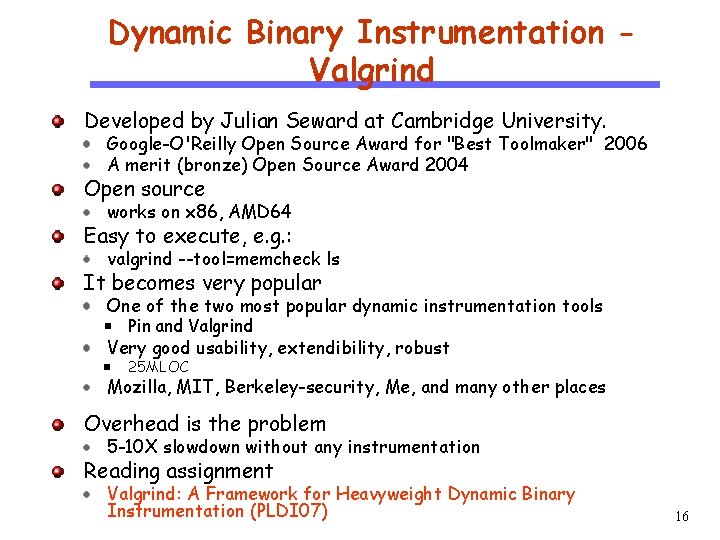
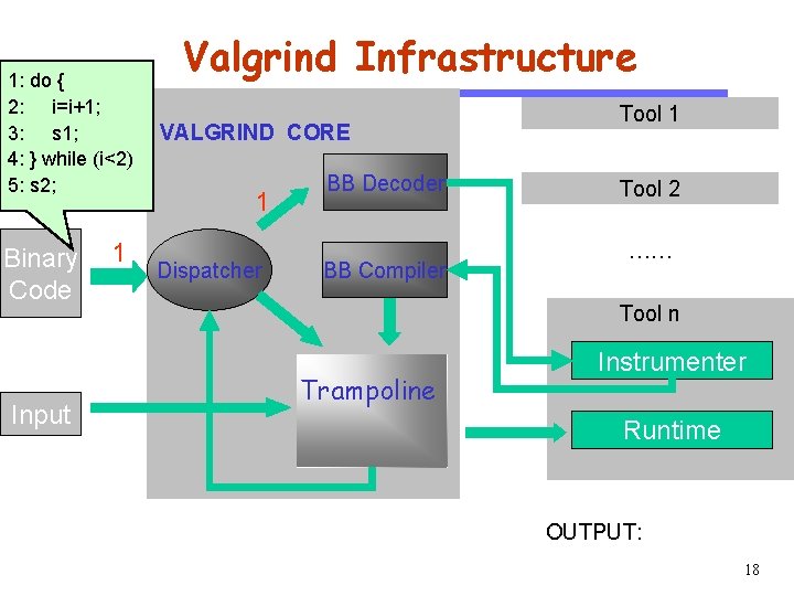
Dynamic Binary Instrumentation Valgrind Developed by Julian Seward at Cambridge University. CS 510 Open source Software Engineering Google-O'Reilly Open Source Award for "Best Toolmaker" 2006 A merit (bronze) Open Source Award 2004 Easy to execute, e. g. : works on x 86, AMD 64 valgrind --tool=memcheck ls It becomes very popular One of the two most popular dynamic instrumentation tools Pin and Valgrind Very good usability, extendibility, robust 25 MLOC Mozilla, MIT, Berkeley-security, Me, and many other places Overhead is the problem 5 -10 X slowdown without any instrumentation Reading assignment Valgrind: A Framework for Heavyweight Dynamic Binary Instrumentation (PLDI 07) 16

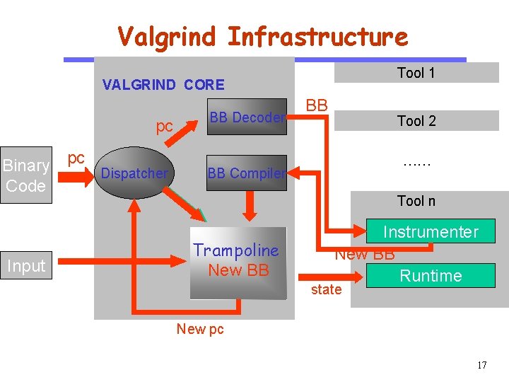
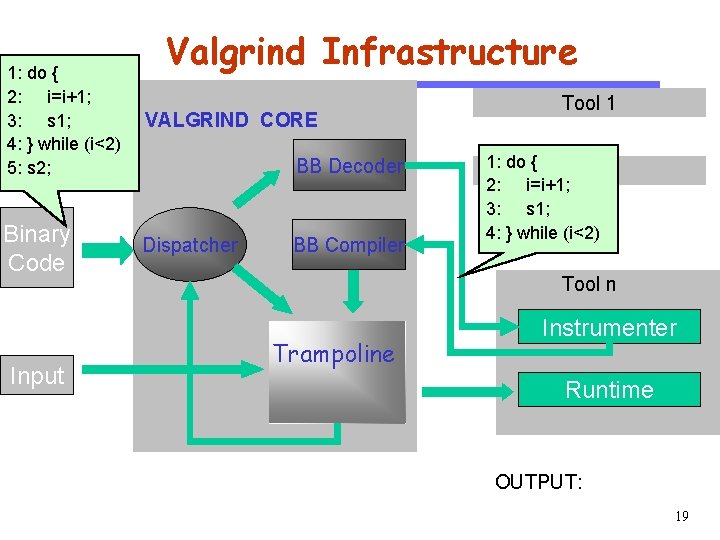
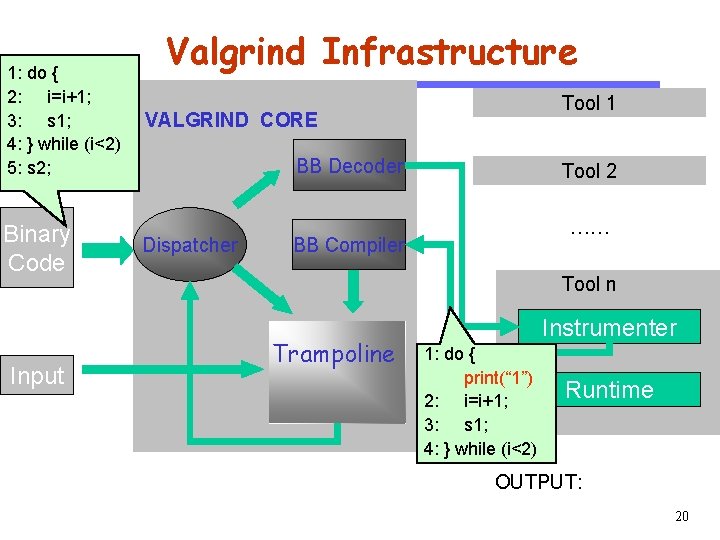
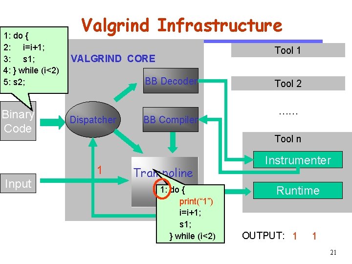
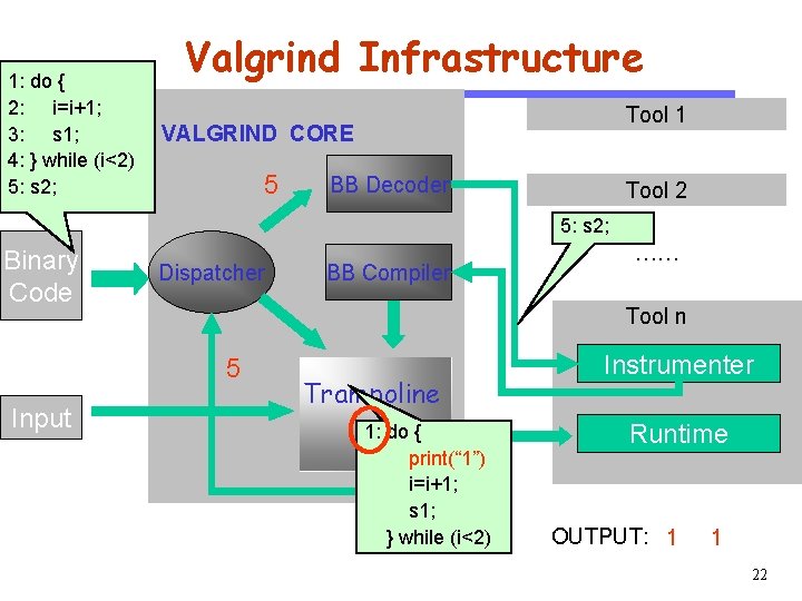
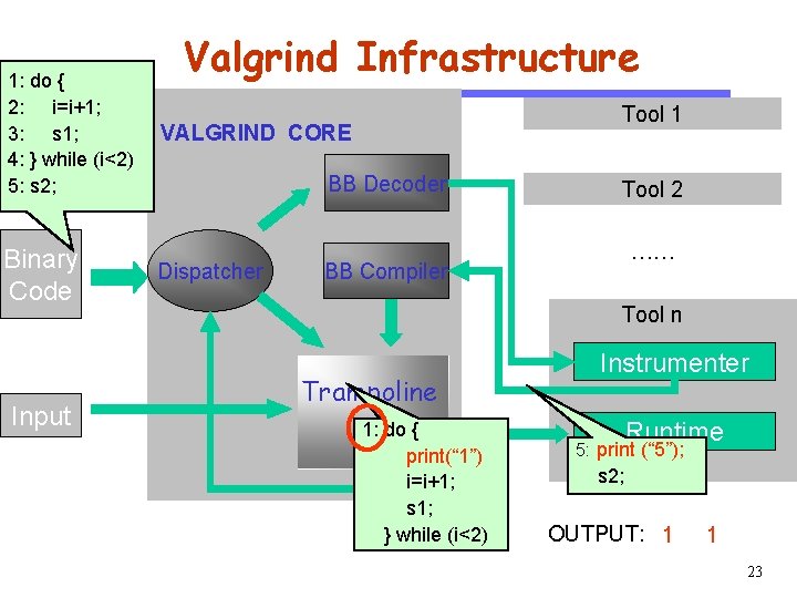
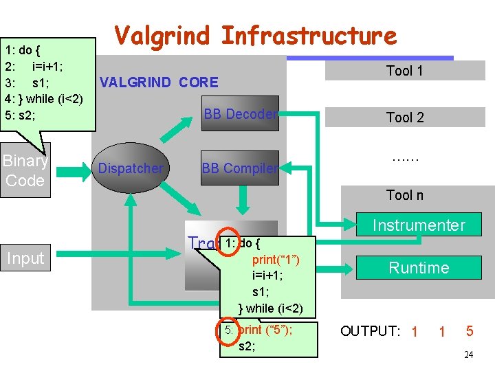
Valgrind Infrastructure Tool 1 VALGRIND CORE CS 510 pc Software Engineering Binary Code Input pc Dispatcher BB Decoder BB Tool 2 …… BB Compiler Tool n Trampoline New BB Instrumenter New BB Runtime state New pc 17

CS 510 1: do { 2: i=i+1; 3: s 1; 4: } while (i<2) 5: s 2; Software Engineering Binary Code Input 1 Valgrind Infrastructure VALGRIND CORE 1 Dispatcher BB Decoder BB Compiler Tool 1 Tool 2 …… Tool n Trampoline Instrumenter Runtime OUTPUT: 18

VALGRIND CORE BB Decoder CS 510 1: do { 2: i=i+1; 3: s 1; 4: } while (i<2) 5: s 2; Valgrind Infrastructure Software Engineering Binary Code Input Dispatcher BB Compiler Tool 1 1: do { Tool 2 2: i=i+1; 3: s 1; …… 4: } while (i<2) Tool n Trampoline Instrumenter Runtime OUTPUT: 19

Software Engineering Binary Code Input Tool 1 VALGRIND CORE BB Decoder CS 510 1: do { 2: i=i+1; 3: s 1; 4: } while (i<2) 5: s 2; Valgrind Infrastructure Dispatcher Tool 2 …… BB Compiler Tool n Trampoline Instrumenter 1: do { print(“ 1”) 2: i=i+1; 3: s 1; 4: } while (i<2) Runtime OUTPUT: 20

Software Engineering Binary Code Input Tool 1 VALGRIND CORE BB Decoder CS 510 1: do { 2: i=i+1; 3: s 1; 4: } while (i<2) 5: s 2; Valgrind Infrastructure Dispatcher BB Compiler Tool 2 …… Tool n 1 Trampoline 1: do { print(“ 1”) i=i+1; s 1; } while (i<2) Instrumenter Runtime OUTPUT: 1 1 21

Software Engineering Binary Code Input Tool 1 VALGRIND CORE 5 CS 510 1: do { 2: i=i+1; 3: s 1; 4: } while (i<2) 5: s 2; Valgrind Infrastructure BB Decoder Tool 2 5: s 2; Dispatcher BB Compiler …… Tool n 5 Trampoline 1: do { print(“ 1”) i=i+1; s 1; } while (i<2) Instrumenter Runtime OUTPUT: 1 1 22

Software Engineering Binary Code Input Tool 1 VALGRIND CORE BB Decoder CS 510 1: do { 2: i=i+1; 3: s 1; 4: } while (i<2) 5: s 2; Valgrind Infrastructure Dispatcher Tool 2 …… BB Compiler Tool n Trampoline 1: do { print(“ 1”) i=i+1; s 1; } while (i<2) Instrumenter Runtime 5: print (“ 5”); s 2; OUTPUT: 1 1 23

Software Engineering Binary Code Input Tool 1 VALGRIND CORE BB Decoder CS 510 1: do { 2: i=i+1; 3: s 1; 4: } while (i<2) 5: s 2; Valgrind Infrastructure Dispatcher BB Compiler Tool 2 …… Tool n 1: do { Trampoline print(“ 1”) i=i+1; s 1; } while (i<2) 5: print (“ 5”); s 2; Instrumenter Runtime OUTPUT: 1 1 5 24

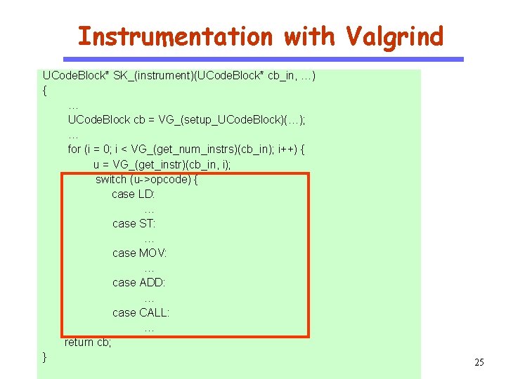
Instrumentation with Valgrind CS 510 Software Engineering UCode. Block* SK_(instrument)(UCode. Block* cb_in, …) { … UCode. Block cb = VG_(setup_UCode. Block)(…); … for (i = 0; i < VG_(get_num_instrs)(cb_in); i++) { u = VG_(get_instr)(cb_in, i); switch (u->opcode) { case LD: … case ST: … case MOV: … case ADD: … case CALL: … return cb; } 25

Outline CS 510 Software Engineering What is tracing. Why tracing. How to trace. Reducing trace size. 26

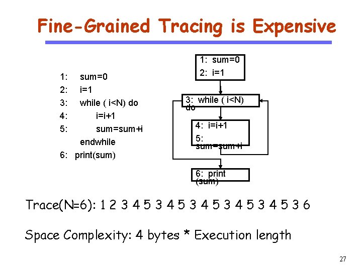
Fine-Grained Tracing is Expensive CS 510 Software Engineering 1: 2: 3: 4: 5: sum=0 i=1 while ( i<N) do i=i+1 sum=sum+i endwhile 6: print(sum) 1: sum=0 2: i=1 3: while ( i<N) do 4: i=i+1 5: sum=sum+i 6: print (sum) Trace(N=6): 1 2 3 4 5 3 4 5 3 6 Space Complexity: 4 bytes * Execution length 27

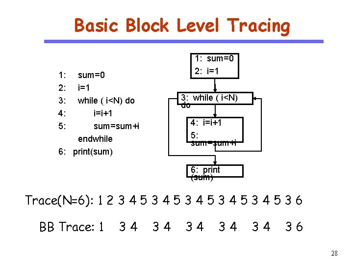
Basic Block Level Tracing 1: sum=0 2: i=1 CS 510 Software Engineering 1: 2: 3: 4: 5: sum=0 i=1 while ( i<N) do i=i+1 sum=sum+i endwhile 6: print(sum) 3: while ( i<N) do 4: i=i+1 5: sum=sum+i 6: print (sum) Trace(N=6): 1 2 3 4 5 3 4 5 3 6 BB Trace: 1 34 34 34 36 28

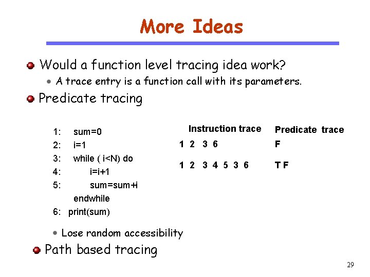
More Ideas Would a function level tracing idea work? A trace entry is a function call with its parameters. CS 510 Predicate tracing Software Engineering 1: 2: 3: 4: 5: sum=0 i=1 while ( i<N) do i=i+1 sum=sum+i endwhile 6: print(sum) Instruction trace Predicate trace 1 2 3 6 F 1 2 3 4 5 3 6 TF Lose random accessibility Path based tracing 29

Intel PT https: //software. intel. com/enus/blogs/2013/09/18/processor-tracing CS 510 Software Engineering 07 六月 2021 30

Program Slicing Xiangyu Zhang

Outline CS 510 Software Engineering What is slicing. Why slicing. Static slicing. Dynamic slicing. Data dependence detection Control dependence detection Slicing algorithms (forward vs. backward) Chopping 32

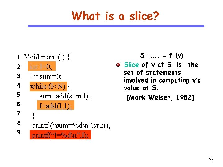
What is a slice? CS 510 1 Software Engineering 2 3 4 5 6 7 8 9 Void main ( ) { int I=0; int sum=0; while (I<N) { sum=add(sum, I); I=add(I, 1); } printf (“sum=%dn”, sum); printf(“I=%dn”, I); S: …. = f (v) Slice of v at S is the set of statements involved in computing v’s value at S. [Mark Weiser, 1982] 33

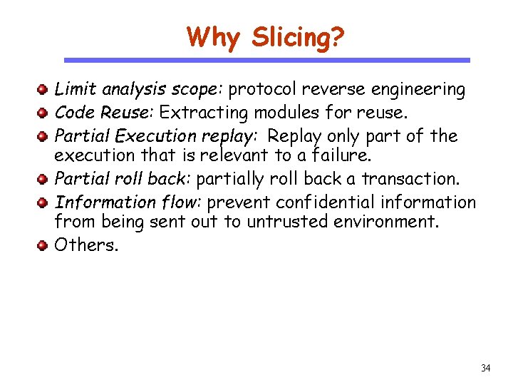
Why Slicing? CS 510 Software Engineering Limit analysis scope: protocol reverse engineering Code Reuse: Extracting modules for reuse. Partial Execution replay: Replay only part of the execution that is relevant to a failure. Partial roll back: partially roll back a transaction. Information flow: prevent confidential information from being sent out to untrusted environment. Others. 34

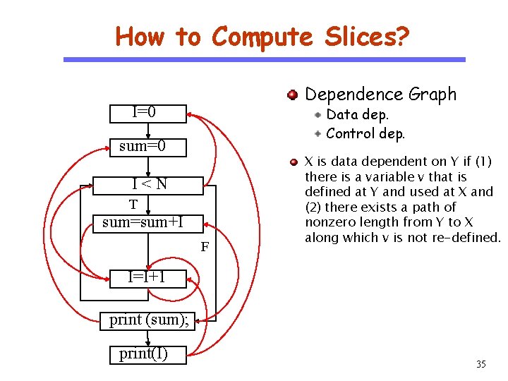
How to Compute Slices? Dependence Graph I=0 CS 510 Data dep. Control dep. Software Engineering sum=0 I<N T sum=sum+I F X is data dependent on Y if (1) there is a variable v that is defined at Y and used at X and (2) there exists a path of nonzero length from Y to X along which v is not re-defined. I=I+1 print (sum); print(I) 35

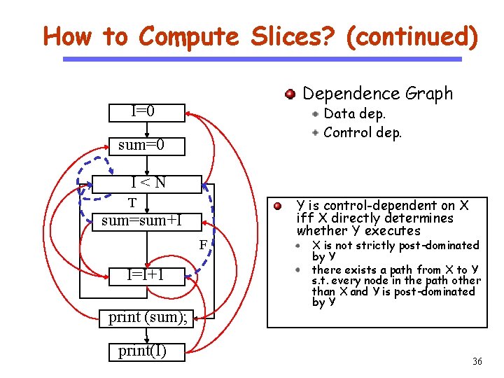
How to Compute Slices? (continued) Dependence Graph I=0 CS 510 Data dep. Control dep. Software Engineering sum=0 I<N T sum=sum+I F I=I+1 print (sum); print(I) Y is control-dependent on X iff X directly determines whether Y executes X is not strictly post-dominated by Y there exists a path from X to Y s. t. every node in the path other than X and Y is post-dominated by Y 36

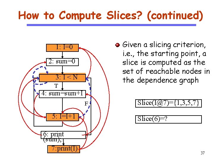
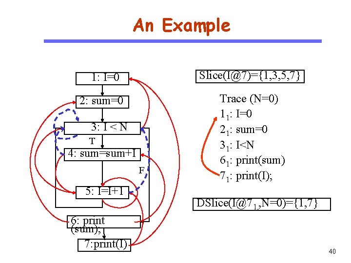
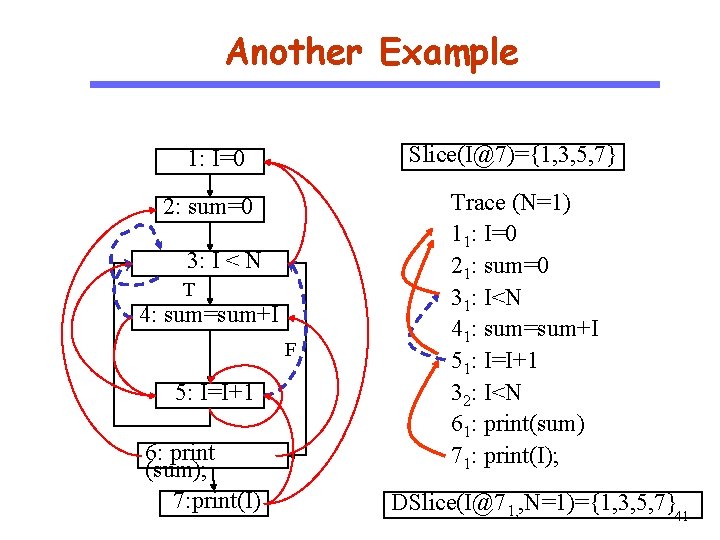
How to Compute Slices? (continued) Given a slicing criterion, i. e. , the starting point, a slice is computed as the set of reachable nodes in the dependence graph 1: I=0 CS 510 Software Engineering 2: sum=0 3: I < N T 4: sum=sum+I F 5: I=I+1 6: print (sum); 7: print(I) Slice(I@7)={1, 3, 5, 7} Slice(6)=? 37

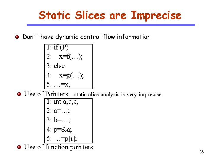
Static Slices are Imprecise Don’t have dynamic control flow information CS 510 Software Engineering 1: if (P) 2: x=f(…); 3: else 4: x=g(…); 5. …=x; Use of Pointers – static alias analysis is very imprecise 1: int a, b, c; 2: a=…; 3: b=…; 4: p=&a; 5: …=p[i]; Use of function pointers 38

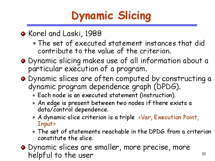
Dynamic Slicing CS 510 Software Engineering Korel and Laski, 1988 The set of executed statement instances that did contribute to the value of the criterion. Dynamic slicing makes use of all information about a particular execution of a program. Dynamic slices are often computed by constructing a dynamic program dependence graph (DPDG). Each node is an executed statement (instruction). An edge is present between two nodes if there exists a data/control dependence. A dynamic slice criterion is a triple <Var, Execution Point, Input> The set of statements reachable in the DPDG from a criterion constitute the slice. Dynamic slices are smaller, more precise, more helpful to the user 39

An Example Slice(I@7)={1, 3, 5, 7} 1: I=0 CS 510 Software Engineering 2: sum=0 3: I < N T 4: sum=sum+I F 5: I=I+1 6: print (sum); 7: print(I) Trace (N=0) 11: I=0 21: sum=0 31: I<N 61: print(sum) 71: print(I); DSlice(I@71, , N=0)={1, 7} 40

Another Example Slice(I@7)={1, 3, 5, 7} 1: I=0 CS 510 Software Engineering 2: sum=0 3: I < N T 4: sum=sum+I F 5: I=I+1 6: print (sum); 7: print(I) Trace (N=1) 11: I=0 21: sum=0 31: I<N 41: sum=sum+I 51: I=I+1 32: I<N 61: print(sum) 71: print(I); DSlice(I@71, , N=1)={1, 3, 5, 7}41

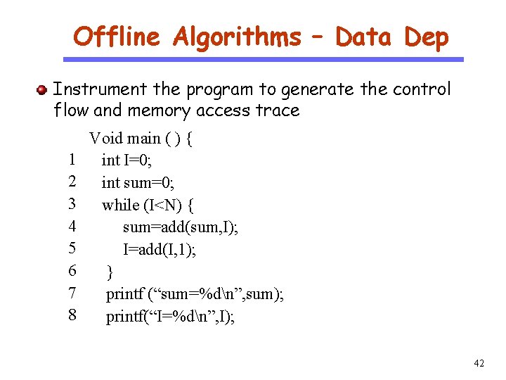
Offline Algorithms – Data Dep CS 510 Instrument the program to generate the control flow and memory access trace Software Engineering 1 2 3 4 5 6 7 8 Void main ( ) { int I=0; int sum=0; while (I<N) { sum=add(sum, I); I=add(I, 1); } printf (“sum=%dn”, sum); printf(“I=%dn”, I); 42

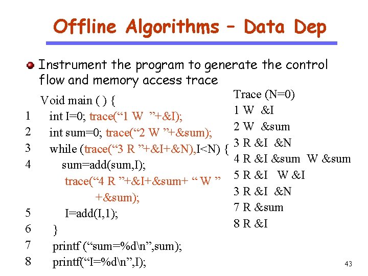
Offline Algorithms – Data Dep CS 510 Software Engineering 1 2 3 4 5 6 7 8 Instrument the program to generate the control flow and memory access trace Trace (N=0) Void main ( ) { 1 W &I int I=0; trace(“ 1 W ”+&I); 2 W &sum int sum=0; trace(“ 2 W ”+&sum); while (trace(“ 3 R ”+&I+&N), I<N) { 3 R &I &N 4 R &I &sum W &sum sum=add(sum, I); trace(“ 4 R ”+&I+&sum+ “ W ” 5 R &I W &I 3 R &I &N +&sum); 7 R &sum I=add(I, 1); 8 R &I } printf (“sum=%dn”, sum); printf(“I=%dn”, I); 43

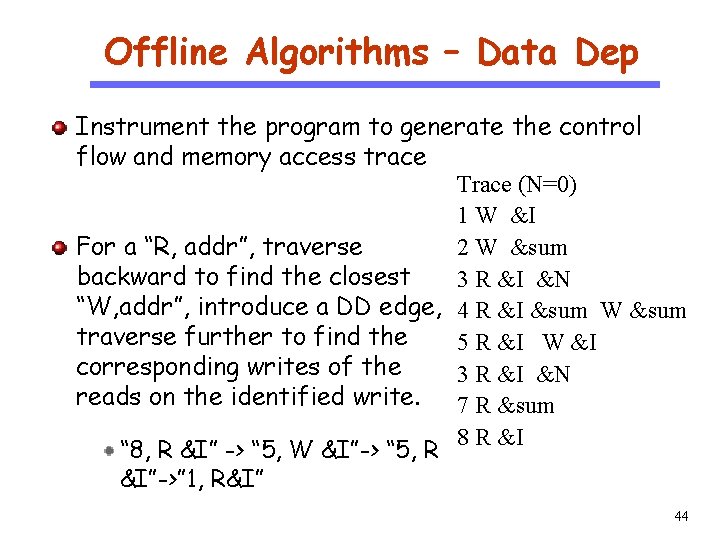
Offline Algorithms – Data Dep CS 510 Software Engineering Instrument the program to generate the control flow and memory access trace Trace (N=0) 1 W &I 2 W &sum For a “R, addr”, traverse backward to find the closest 3 R &I &N “W, addr”, introduce a DD edge, 4 R &I &sum W &sum traverse further to find the 5 R &I W &I corresponding writes of the 3 R &I &N reads on the identified write. 7 R &sum 8 R &I “ 8, R &I” -> “ 5, W &I”-> “ 5, R &I”->” 1, R&I” 44

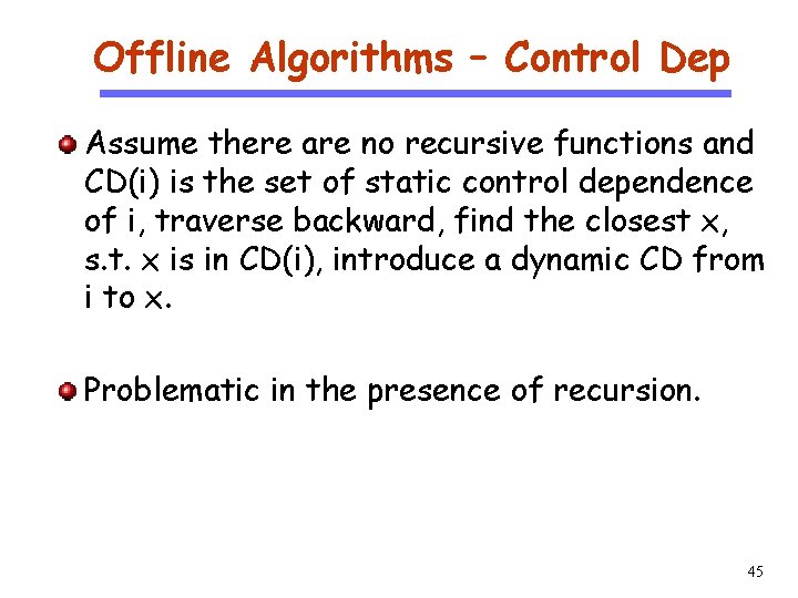
Offline Algorithms – Control Dep CS 510 Software Engineering Assume there are no recursive functions and CD(i) is the set of static control dependence of i, traverse backward, find the closest x, s. t. x is in CD(i), introduce a dynamic CD from i to x. Problematic in the presence of recursion. 45

Efficiently Computing Dynamic Dependences CS 510 Software Engineering The previous mentioned graph construction algorithm implies offline traversals of long memory reference and control flow traces Efficient online algorithms Online data dependence detection. Online control dependence detection. 46

Efficient Data Dependence Detection Basic idea CS 510 i: x=… => hashmap[x]= i j: … =x… => dependence detected j hashmap[x], which is j i Software Engineering Trace (N=1) 11: I=0 21: sum=0 31: I<N 41: sum=sum+I 51: I=I+1 32: I<N 61: print(sum) 71: print(I); Hash. Map I: 11 Data Dep. I: 11 sum: 21 I: 11 sum: 41 I: 51 sum: 41 31 41 51 32 61 71 hashmap[I]=11 hashmap[sum]=21 hashmap[I]=11 hashmap[I]=51 hashmap[sum]=41 hashmap[I]=51 47

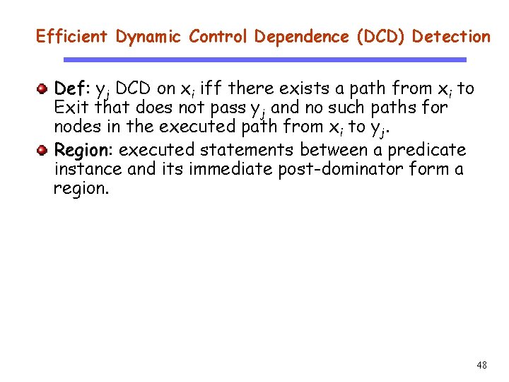
Efficient Dynamic Control Dependence (DCD) Detection CS 510 Software Engineering Def: yj DCD on xi iff there exists a path from xi to Exit that does not pass yj and no such paths for nodes in the executed path from xi to yj. Region: executed statements between a predicate instance and its immediate post-dominator form a region. 48

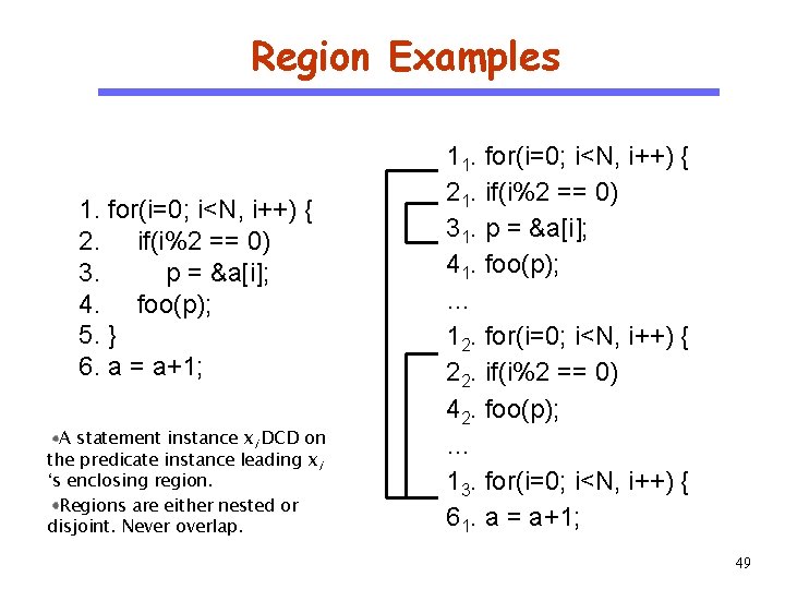
Region Examples CS 510 Software Engineering 1. for(i=0; i<N, i++) { 2. if(i%2 == 0) 3. p = &a[i]; 4. foo(p); 5. } 6. a = a+1; A statement instance xi DCD on the predicate instance leading xi ‘s enclosing region. Regions are either nested or disjoint. Never overlap. 11. for(i=0; i<N, i++) { 21. if(i%2 == 0) 31. p = &a[i]; 41. foo(p); … 12. for(i=0; i<N, i++) { 22. if(i%2 == 0) 42. foo(p); … 13. for(i=0; i<N, i++) { 61. a = a+1; 49

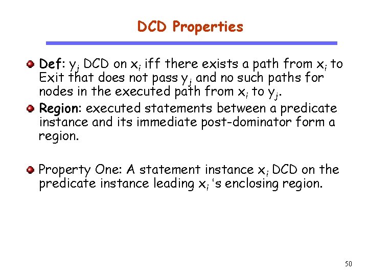
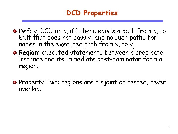
DCD Properties CS 510 Software Engineering Def: yj DCD on xi iff there exists a path from xi to Exit that does not pass yj and no such paths for nodes in the executed path from xi to yj. Region: executed statements between a predicate instance and its immediate post-dominator form a region. Property One: A statement instance xi DCD on the predicate instance leading xi ‘s enclosing region. 50

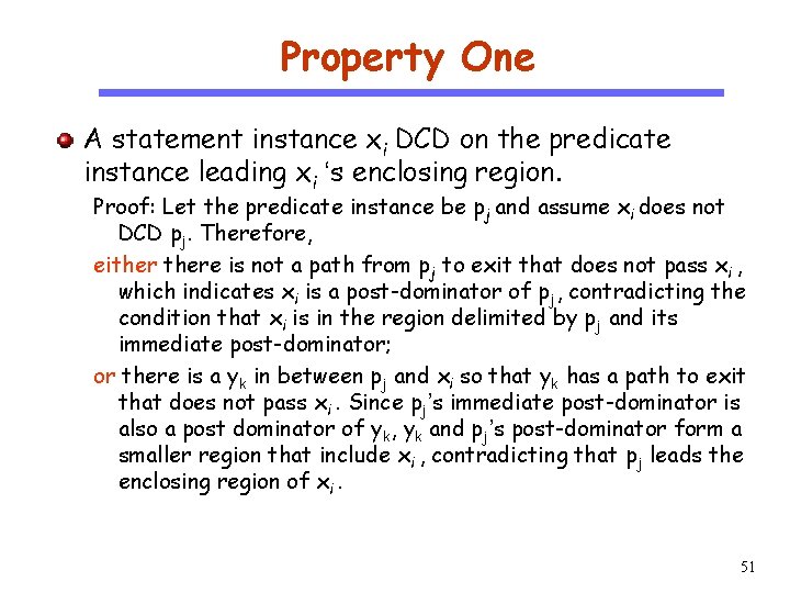
Property One CS 510 A statement instance xi DCD on the predicate instance leading xi ‘s enclosing region. Software Engineering Proof: Let the predicate instance be pj and assume xi does not DCD pj. Therefore, eithere is not a path from pj to exit that does not pass xi , which indicates xi is a post-dominator of pj, contradicting the condition that xi is in the region delimited by pj and its immediate post-dominator; or there is a yk in between pj and xi so that yk has a path to exit that does not pass xi. Since pj’s immediate post-dominator is also a post dominator of yk, yk and pj’s post-dominator form a smaller region that include xi , contradicting that pj leads the enclosing region of xi. 51

DCD Properties CS 510 Software Engineering Def: yj DCD on xi iff there exists a path from xi to Exit that does not pass yj and no such paths for nodes in the executed path from xi to yj. Region: executed statements between a predicate instance and its immediate post-dominator form a region. Property Two: regions are disjoint or nested, never overlap. 52

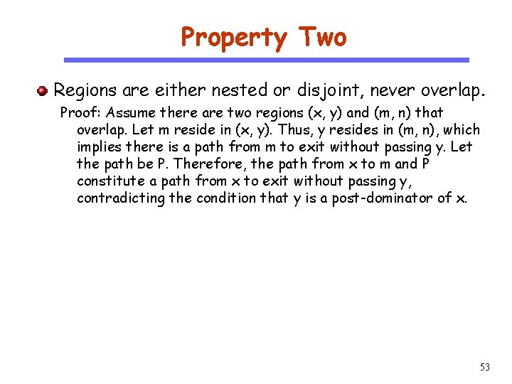
Property Two Regions are either nested or disjoint, never overlap. CS 510 Software Engineering Proof: Assume there are two regions (x, y) and (m, n) that overlap. Let m reside in (x, y). Thus, y resides in (m, n), which implies there is a path from m to exit without passing y. Let the path be P. Therefore, the path from x to m and P constitute a path from x to exit without passing y, contradicting the condition that y is a post-dominator of x. 53

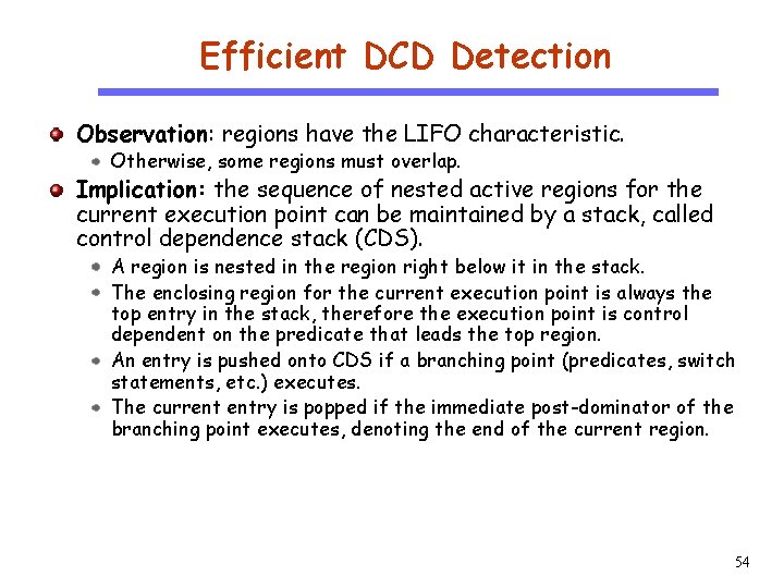
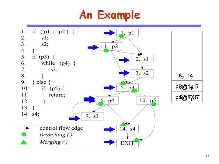
Efficient DCD Detection Observation: regions have the LIFO characteristic. Otherwise, some regions must overlap. CS 510 Software Engineering Implication: the sequence of nested active regions for the current execution point can be maintained by a stack, called control dependence stack (CDS). A region is nested in the region right below it in the stack. The enclosing region for the current execution point is always the top entry in the stack, therefore the execution point is control dependent on the predicate that leads the top region. An entry is pushed onto CDS if a branching point (predicates, switch statements, etc. ) executes. The current entry is popped if the immediate post-dominator of the branching point executes, denoting the end of the current region. 54

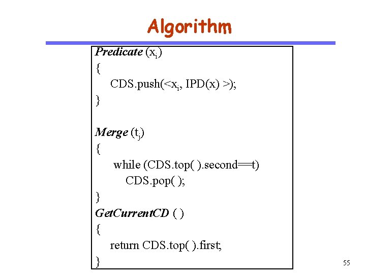
Algorithm CS 510 Predicate (xi) { CDS. push(<xi, IPD(x) >); } Software Engineering Merge (tj) { while (CDS. top( ). second==t) CDS. pop( ); } Get. Current. CD ( ) { return CDS. top( ). first; } 55

An Example CS 510 Software Engineering 62, 14 p 2@1 61, 14 1, 5 p 1@1 51, EXIT 1, 5 56

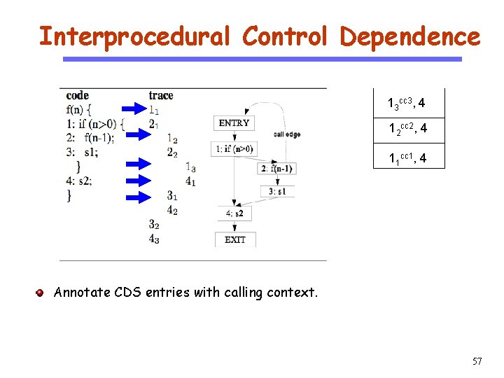
Interprocedural Control Dependence 13 cc 3, 4 CS 510 12 cc 2, 4 Software Engineering 11 cc 1, 4 Annotate CDS entries with calling context. 57

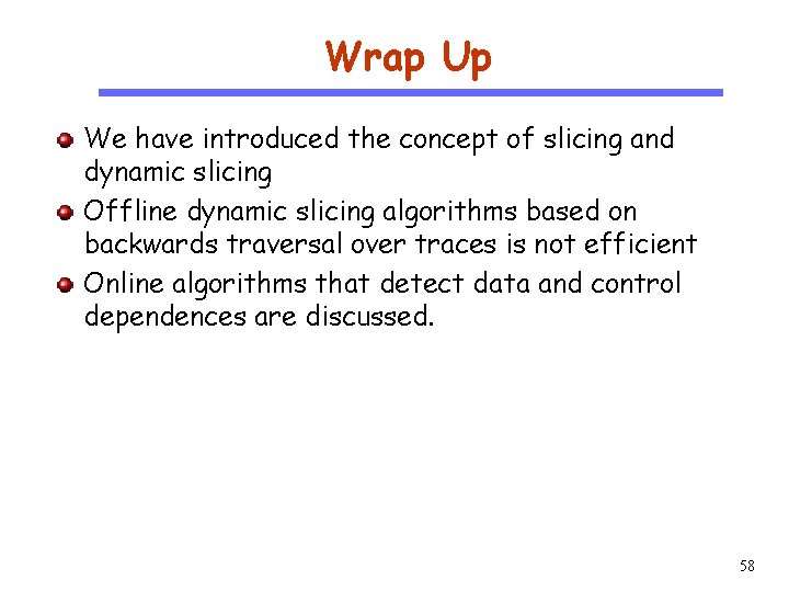
Wrap Up CS 510 Software Engineering We have introduced the concept of slicing and dynamic slicing Offline dynamic slicing algorithms based on backwards traversal over traces is not efficient Online algorithms that detect data and control dependences are discussed. 58

Forward Dynamic Slice Computation CS 510 The approaches we have discussed so far are backwards. Software Engineering Dependence graphs are traversed backwards from a slicing criterion. The space complexity is O (execution length). Forward computation A slice is represented as a set of statements that are involved in computing the value of the slicing criterion. A slice is always maintained for a variable. 59

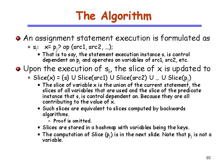
The Algorithm An assignment statement execution is formulated as si: x= pj? op (src 1, src 2, …); CS 510 That is to say, the statement execution instance s i is control dependent on pj and operates on variables of src 1, src 2, etc. Software Engineering Upon the execution of si, the slice of x is updated to Slice(x) = {s} U Slice(src 1) U Slice(src 2) U … U Slice(p j) The slice of variable x is the union of the current statement, the slices of all variables that are used and the slice of the predicate instance that si is control dependent on. Because they are all contributing to the value of x. Such slices are equivalent to slices computed by backwards algorithms. – Proof is omitted. Slices are stored in a hashmap with variables being the keys. The computation of Slice (pj) is in the next slide. Note that pj is not a variable. 60

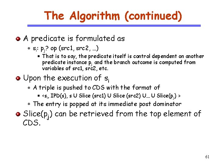
The Algorithm (continued) A predicate is formulated as CS 510 si: pj? op (src 1, src 2, …) Software Engineering That is to say, the predicate itself is control dependent on another predicate instance pj and the branch outcome is computed from variables of src 1, src 2, etc. Upon the execution of si A triple is pushed to CDS with the format of <si, IPD(s), s U Slice (src 1) U Slice (src 2) U… U Slice(p j) > The entry is popped at its immediate post dominator Slice(pj) can be retrieved from the top element of CDS. 61

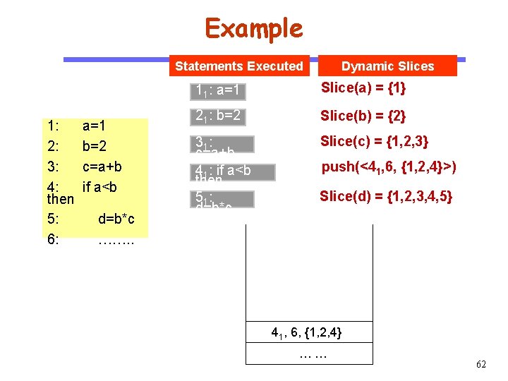
Example Statements Executed CS 510 Software Engineering 1: 2: 3: 4: then 5: 6: a=1 b=2 c=a+b if a<b d=b*c ……. . Dynamic Slices 11: a=1 Slice(a) = {1} 21: b=2 Slice(b) = {2} 31 : c=a+b 41: if a<b then 51 : d=b*c Slice(c) = {1, 2, 3} push(<41, 6, {1, 2, 4}>) Slice(d) = {1, 2, 3, 4, 5} 41, 6, {1, 2, 4} …… 62

Properties CS 510 The slices are equivalent to those computed by backwards algorithms The proof is omitted. Software Engineering The space complexity is bounded O ( (# of variables + MAX_CDS_DEPTH) * # of statements) Efficiency relies on the hash map implementation and set operations. A cost-effective implementation will be discussed later in cs 510. 63

Extending Slicing CS 510 Software Engineering Essentially, slicing is an orthogonal approach to isolate part of a program (execution) giving certain criterion. Mutations of slicing Event slicing – intrusion detection, execution fast forwarding, understanding network protocol, malware replayer. Forward slicing. Chopping. Probabilistic slicing. 64

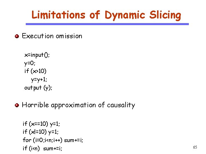
Limitations of Dynamic Slicing Execution omission CS 510 Software Engineering x=input(); y=0; if (x>10) y=y+1; output (y); Horrible approximation of causality if (x==10) y=1; if (x!=10) y=1; for (i=0; i<n; i++) sum+=i; if (i<n) sum+=i; 65

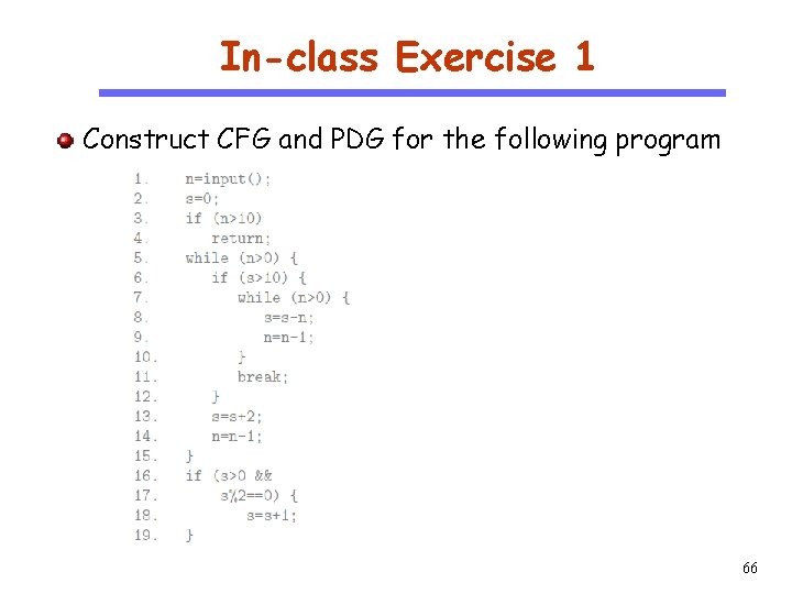
In-class Exercise 1 Construct CFG and PDG for the following program CS 510 Software Engineering 66

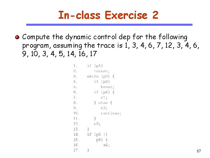
In-class Exercise 2 CS 510 Compute the dynamic control dep for the following program, assuming the trace is 1, 3, 4, 6, 7, 12, 3, 4, 6, 9, 10, 3, 4, 5, 14, 16, 17 Software Engineering 67

Discussion What research projects have you done in the past that use dynamic analysis? CS 510 Software Engineering What are the challenges in those projects and how do you address those challenges? How to quantify dependencies? (First introduce yourself and your research) 68