Dynamic observers for sensor faults detection and diagnosis

Dynamic observers for sensor faults detection and diagnosis Presented by: Pertew, A. M. Supervised by: Dr. Marquez, H. J. Dr. Zhao, Q.

Outline • • • Introduction to Fault Detection & Diagnosis (FDD) A dynamical observer approach for sensor FDD Narrow frequency band sensor faults The low frequency range case – an H∞ approach Simulation results Conclusion Outline ( 1/18)

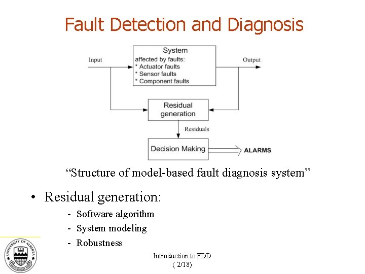
Fault Detection and Diagnosis “Structure of model-based fault diagnosis system” • Residual generation: - Software algorithm - System modeling - Robustness Introduction to FDD ( 2/18)

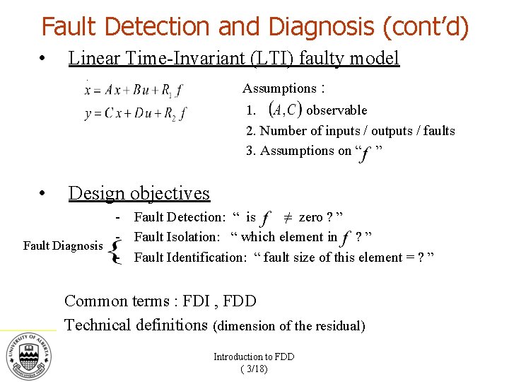
Fault Detection and Diagnosis (cont’d) • Linear Time-Invariant (LTI) faulty model Assumptions : 1. observable 2. Number of inputs / outputs / faults 3. Assumptions on “ ” • Design objectives - Fault Detection: “ is ≠ zero ? ” - Fault Isolation: “ which element in ? ” Fault Diagnosis - Fault Identification: “ fault size of this element = ? ” Common terms : FDI , FDD Technical definitions (dimension of the residual) Introduction to FDD ( 3/18)

Fault Detection and Diagnosis (cont’d) • Important work: - Luenberger and Kalman (observer) Beard (unidirectional residual) Frank and Ding (dedicated observer, optimization) Watanabe (Unknown Input Observer “UIO”) Patton and Chen (eigen structure assignment) Introduction to FDD ( 4/18)

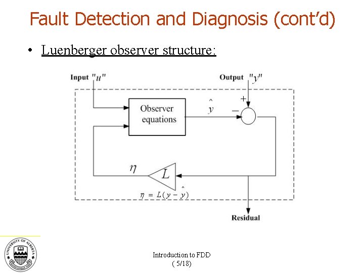
Fault Detection and Diagnosis (cont’d) • Luenberger observer structure: Introduction to FDD ( 5/18)

Outline ü Introduction to Fault Detection & Diagnosis (FDD) • A dynamical observer approach for sensor FDD • Narrow frequency band sensor faults • The low frequency range case – an H∞ approach • Simulation results • Conclusion

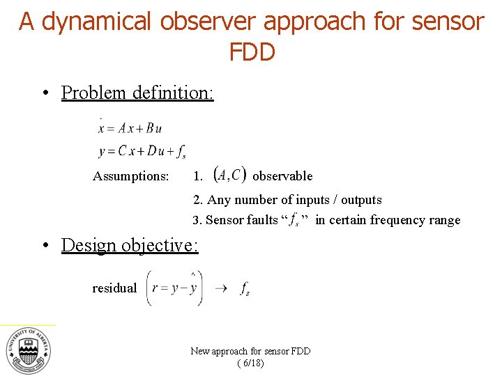
A dynamical observer approach for sensor FDD • Problem definition: Assumptions: 1. observable 2. Any number of inputs / outputs 3. Sensor faults “ ” in certain frequency range • Design objective: residual New approach for sensor FDD ( 6/18)

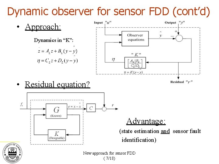
Dynamic observer for sensor FDD (cont’d) • Approach: Dynamics in “K”: • Residual equation? Advantage: (state estimation and sensor fault identification) New approach for sensor FDD ( 7/18)

Outline ü Introduction to Fault Detection & Diagnosis (FDD) ü A dynamical observer approach for sensor FDD • Narrow frequency band sensor faults • The low frequency range case – an H∞ approach • Simulation results • Conclusion

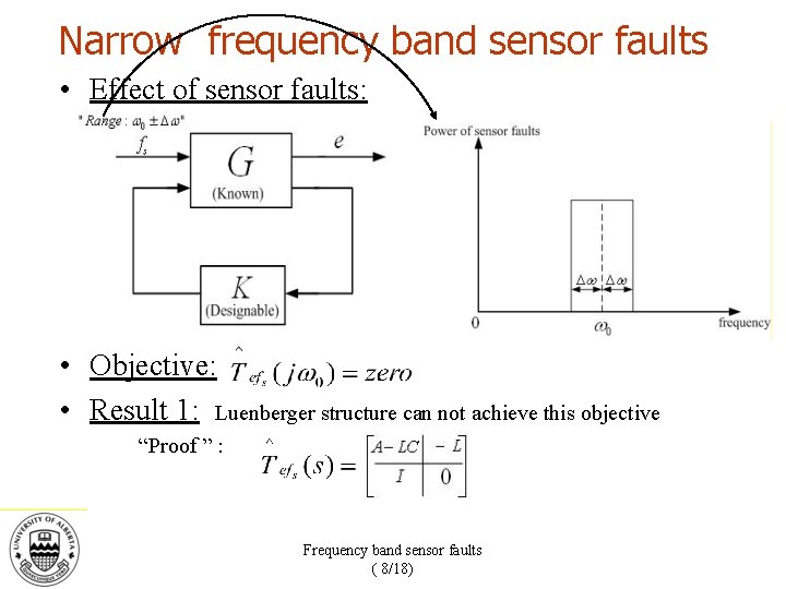
Narrow frequency band sensor faults • Effect of sensor faults: • Objective: • Result 1: Luenberger structure can not achieve this objective “Proof ” : Frequency band sensor faults ( 8/18)

Frequency band sensor faults (cont’d) • Dynamic case: • • Result 2: Result 3: and are invertible “Design of ” Example: 0 = 2 rad/sec , n = 2 , p = 1 1) 2) 3) and let Solve for and “ 2 np” equations in “ 2 np”unknowns

Frequency band sensor faults (cont’d) • Conclusion: – Sensor faults of frequency 0 (application: sensor bias, known harmonics in power systems) – State estimation in addition to fault identification (advantage: fault tolerant control) – Dynamic observer outperforms Luenberger observer Frequency band sensor faults ( 10/18)

Outline ü Introduction to Fault Detection & Diagnosis (FDD) ü A dynamical observer approach for sensor FDD ü Narrow frequency band sensor faults • The low frequency range case – an H∞ approach • Simulation results • Conclusion

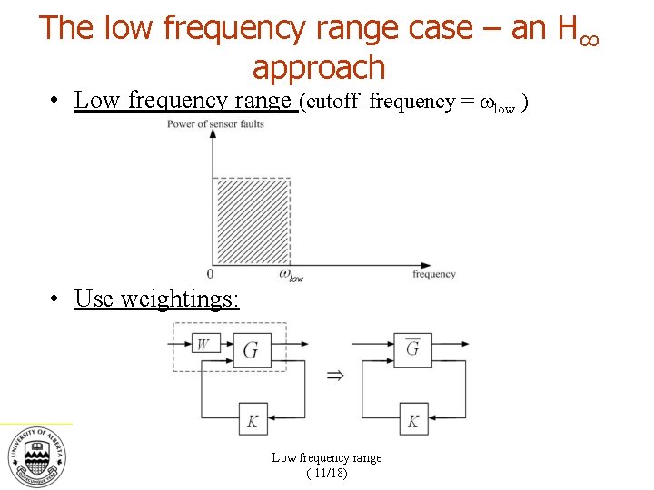
The low frequency range case – an H∞ approach • Low frequency range (cutoff frequency = low ) • Use weightings: Low frequency range ( 11/18)

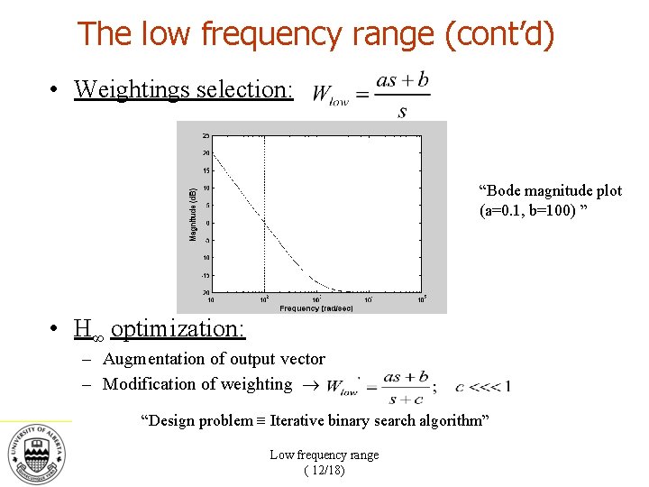
The low frequency range (cont’d) • Weightings selection: “Bode magnitude plot (a=0. 1, b=100) ” • H∞ optimization: – Augmentation of output vector – Modification of weighting “Design problem Iterative binary search algorithm” Low frequency range ( 12/18)

The low frequency range (cont’d) • Conclusion: – H∞ optimization for sensor faults identification (advantage: standard problem, role of dynamic observer) – Weightings selection (different weightings could also be used for different channels) – High frequency range : Low frequency range ( 13/18)

Outline ü Introduction to Fault Detection & Diagnosis (FDD) ü A dynamical observer approach for sensor FDD ü Narrow frequency band sensor faults ü The low frequency range case – an H∞ approach • Simulation results • Conclusion

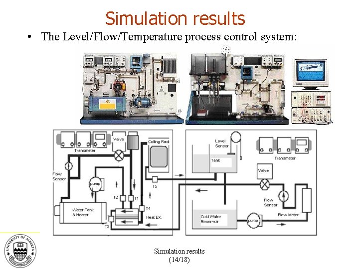
Simulation results • The Level/Flow/Temperature process control system: Simulation results (14/18)

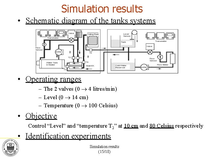
Simulation results • Schematic diagram of the tanks systems • Operating ranges – The 2 valves (0 4 litres/min) – Level (0 14 cm) – Temperature (0 100 Celsius) • Objective Control “Level” and “temperature T 2” at 10 cm and 80 Celsius respectively • Identification experiments Simulation results (15/18)

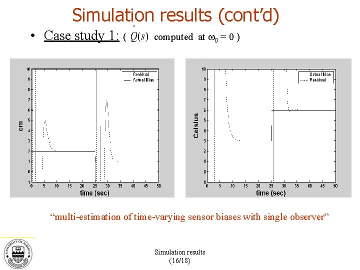
Simulation results (cont’d) • Case study 1: ( computed at 0 = 0 ) “multi-estimation of time-varying sensor biases with single observer” Simulation results (16/18)

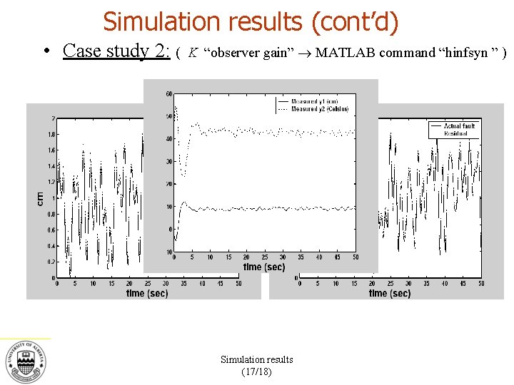
Simulation results (cont’d) • Case study 2: ( K “observer gain” MATLAB command “hinfsyn ” ) Simulation results (17/18)

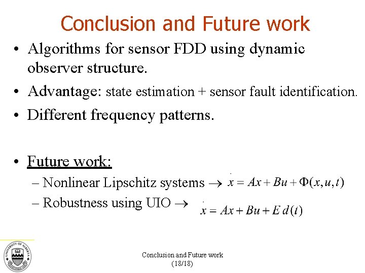
Conclusion and Future work • Algorithms for sensor FDD using dynamic observer structure. • Advantage: state estimation + sensor fault identification. • Different frequency patterns. • Future work: – Nonlinear Lipschitz systems – Robustness using UIO Conclusion and Future work (18/18)

THANK YOU

Questions ?