Dynamic Connectivity Pitfalls and Promises Martin Lindquist Department

Dynamic Connectivity: Pitfalls and Promises Martin Lindquist Department of Biostatistics Johns Hopkins University

Dynamic Connectivity • To date, most resting state f. MRI studies have assumed that the functional connectivity between distinct brain regions is constant across time. • Recently, there has been interest in quantifying possible dynamic changes in connectivity. • Research classifying connectivity into distinct states has demonstrated that the amount of time spent in specific states and the number of transitions between states, vary due to meaningful individual differences (e. g. , age or disease status).

Dynamic Connectivity • Detecting reliable, neuronally-relevant nonstationarities is difficult due to low signal-to-noise ratio, physiological artifacts and variation in signal mean and variance over time. – It is unclear whether observed fluctuations in connectivity should be attributed to neuronal activity or noise. • There remains uncertainty regarding the appropriate analysis strategy to use and how to interpret results.

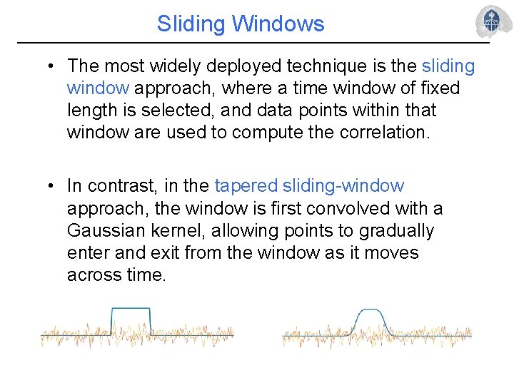
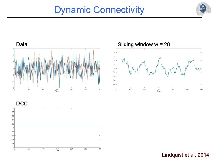
Sliding Windows • The most widely deployed technique is the sliding window approach, where a time window of fixed length is selected, and data points within that window are used to compute the correlation. • In contrast, in the tapered sliding-window approach, the window is first convolved with a Gaussian kernel, allowing points to gradually enter and exit from the window as it moves across time.

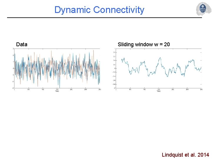
Dynamic Connectivity Data Sliding window w = 20 Lindquist et al. 2014

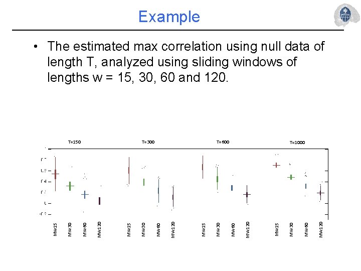
Example • The estimated max correlation using null data of length T, analyzed using sliding windows of lengths w = 15, 30, 60 and 120. MW 120 MW 60 MW 30 MW 15 MW 120 T=1000 MW 60 MW 30 MW 15 MW 120 T=600 MW 60 MW 30 MW 15 MW 120 T=300 MW 60 MW 30 MW 15 T=150

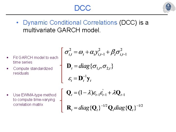
DCC • Dynamic Conditional Correlations (DCC) is a multivariate GARCH model. § Fit GARCH model to each time series § Compute standardized residuals § Use EWMA-type method to compute time-varying correlation matrix

Dynamic Connectivity Data Sliding window w = 20 DCC Lindquist et al. 2014

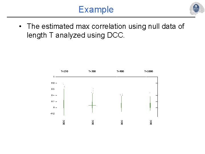
Example T=600 T=1000 DCC T=300 DCC T=150 DCC • The estimated max correlation using null data of length T analyzed using DCC.

Summarizing Information • An interesting aspect about studying dynamic correlations is that it actually increases the number of data points. – The input data is a p×T matrix, where p is the number of regions and T the number of time points. – The output is a series of T p×p matrices summarizing the connectivity at each time point. • Critical need for summary statistics that can be used to find meaningful individual differences.

Summarizing Information • There a number of possible summaries: – The average dynamic correlation and the variability in dynamic correlation in each edge. § If involved in frequent state-changes, edges should exhibit consistently higher variation in correlation. – Connectivity ‘state’ matrices, which are connectivity patterns that subjects tend to return to during the course of an experiment. § Can be summarized based on patterns of connectivity within each state, and used to compute the dwell time each subject spends in a given state.

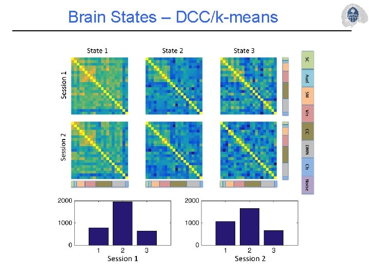
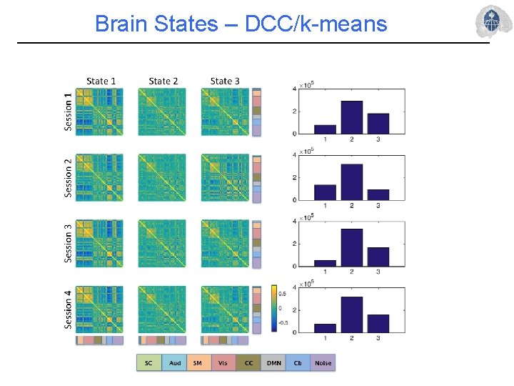
Determining Brain States I • The standard approach towards determining coherent brain states across subjects is to perform clustering on the results of the dynamic connectivity analysis. • Procedure: – Assess dynamic connectivity on each subject – Concatenate the data from all subjects – Perform k-means clustering and let centroids represent ‘brain states’ – Assess dwell time in each state

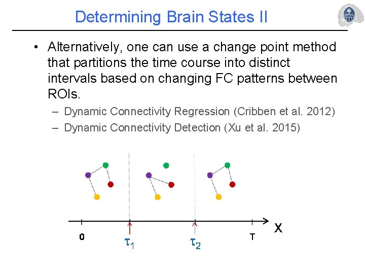
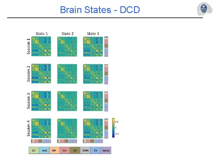
Determining Brain States II • Alternatively, one can use a change point method that partitions the time course into distinct intervals based on changing FC patterns between ROIs. – Dynamic Connectivity Regression (Cribben et al. 2012) – Dynamic Connectivity Detection (Xu et al. 2015)

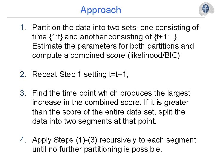
Approach 1. Partition the data into two sets: one consisting of time {1: t} and another consisting of {t+1: T}. Estimate the parameters for both partitions and compute a combined score (likelihood/BIC). 2. Repeat Step 1 setting t=t+1; 3. Find the time point which produces the largest increase in the combined score. If it is greater than the score of the entire data set, split the data into two segments at that point. 4. Apply Steps (1)-(3) recursively to each segment until no further partitioning is possible.

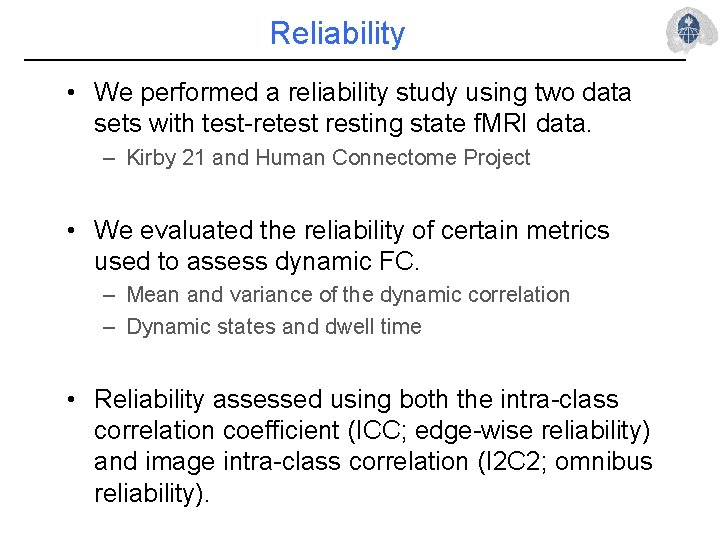
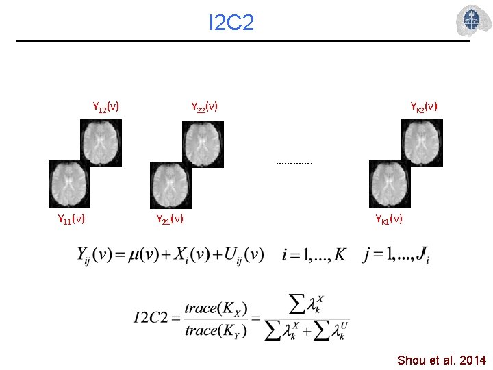
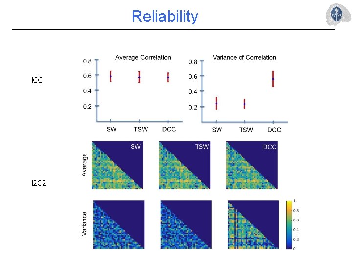
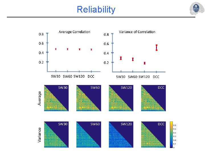
Reliability • We performed a reliability study using two data sets with test-retest resting state f. MRI data. – Kirby 21 and Human Connectome Project • We evaluated the reliability of certain metrics used to assess dynamic FC. – Mean and variance of the dynamic correlation – Dynamic states and dwell time • Reliability assessed using both the intra-class correlation coefficient (ICC; edge-wise reliability) and image intra-class correlation (I 2 C 2; omnibus reliability).

I 2 C 2 Y 12(v) Y 22(v) YK 2(v) …………. Y 11(v) Y 21(v) YK 1(v) Shou et al. 2014

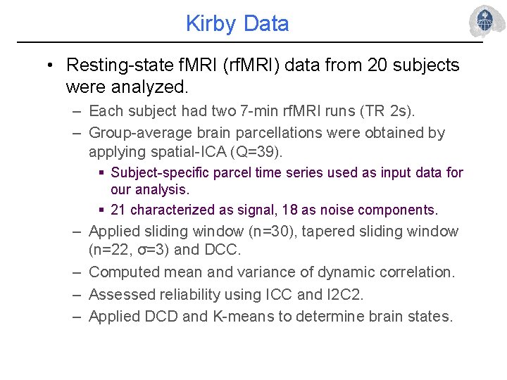
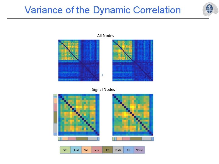
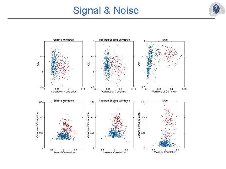
Kirby Data • Resting-state f. MRI (rf. MRI) data from 20 subjects were analyzed. – Each subject had two 7 -min rf. MRI runs (TR 2 s). – Group-average brain parcellations were obtained by applying spatial-ICA (Q=39). § Subject-specific parcel time series used as input data for our analysis. § 21 characterized as signal, 18 as noise components. – Applied sliding window (n=30), tapered sliding window (n=22, σ=3) and DCC. – Computed mean and variance of dynamic correlation. – Assessed reliability using ICC and I 2 C 2. – Applied DCD and K-means to determine brain states.

Reliability ICC I 2 C 2

Variance of the Dynamic Correlation

Signal & Noise

Brain States – DCC/k-means

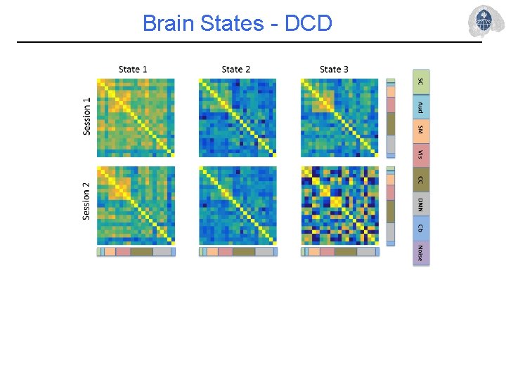
Brain States - DCD

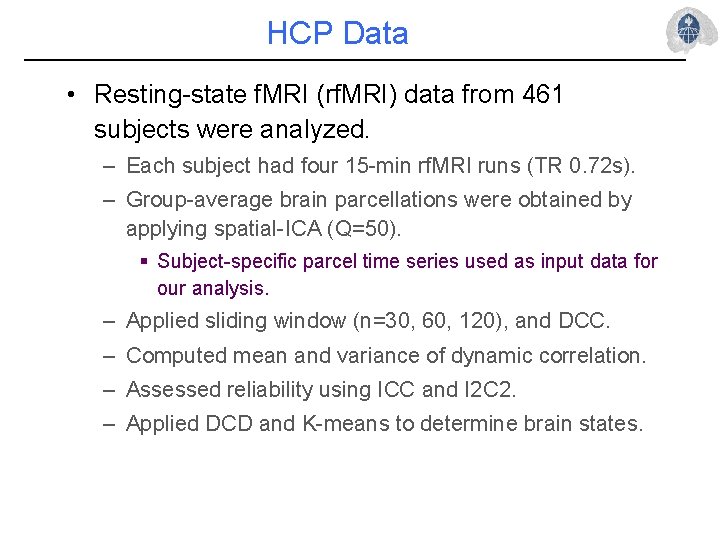
HCP Data • Resting-state f. MRI (rf. MRI) data from 461 subjects were analyzed. – Each subject had four 15 -min rf. MRI runs (TR 0. 72 s). – Group-average brain parcellations were obtained by applying spatial-ICA (Q=50). § Subject-specific parcel time series used as input data for our analysis. – Applied sliding window (n=30, 60, 120), and DCC. – Computed mean and variance of dynamic correlation. – Assessed reliability using ICC and I 2 C 2. – Applied DCD and K-means to determine brain states.

Reliability ICC I 2 C 2

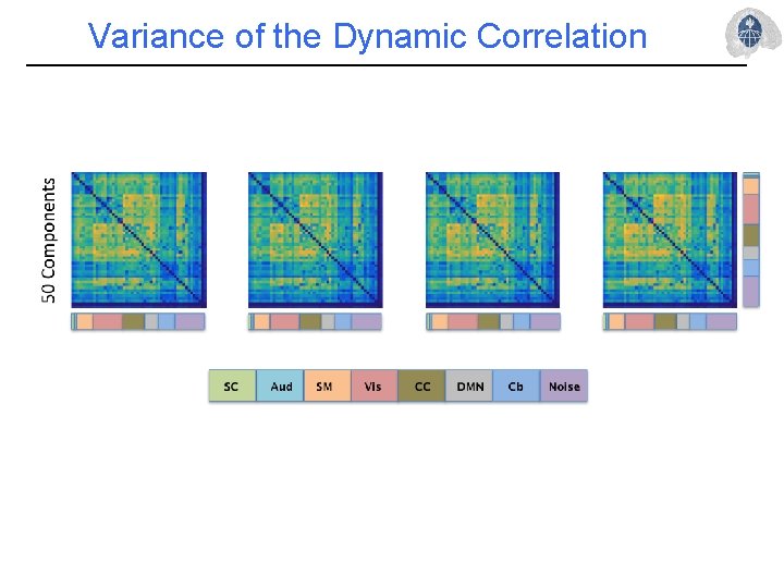
Variance of the Dynamic Correlation

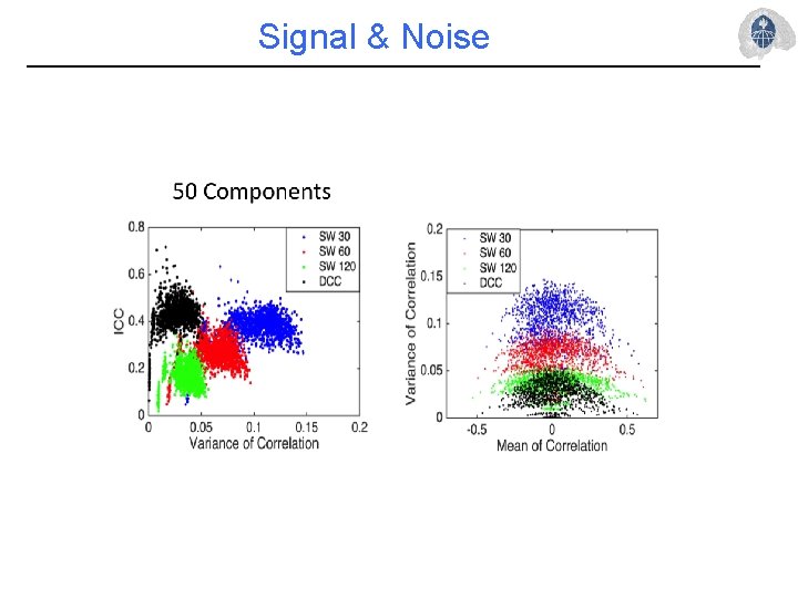
Signal & Noise

Brain States – DCC/k-means

Brain States - DCD

Conclusions • We compared several variants of the slidingwindows technique with a model-based approach. • We evaluated the reproducibility of metrics computed from dynamic FC. – Found moderately strong reproducibility of the average correlation, lower for the variance. § Comparable to other f. MRI analyses (e. g. seed analysis). – DCC provides more reproducible results for the variance and separated signal from non-signal. • Found that we could reliably asses both brain states and dwell time.

Thanks • Joint work with Anita Barber, Ann Choe, Jessica Cohen, Mary-Beth Nebel, Yuting Xu, and Brian Caffo. • References: Martin Lindquist, Yuting Xu, Mary Beth Nebel, and Brain Caffo (2014). Evaluating Dynamic Bivariate Correlations in Resting-state f. MRI: A comparison study and a new approach. Neuro. Image, 101, 531– 546. • Funding: NIH - R 01 EB 016061

Thanks • Thank you for your attention. • Coursera f. MRI class available on demand.