Dynamic Causal Model for evoked responses in MEGEEG

Dynamic Causal Model for evoked responses in MEG/EEG Rosalyn Moran

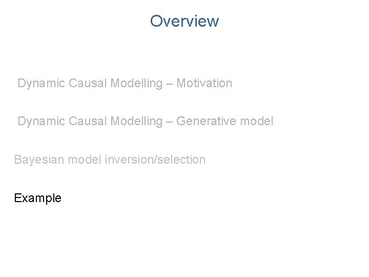
Overview Dynamic Causal Modelling – Motivation Dynamic Causal Modelling – Generative model Bayesian model inversion/selection Example

Overview Dynamic Causal Modelling – Motivation Dynamic Causal Modelling – Generative model Bayesian model inversion/selection Example

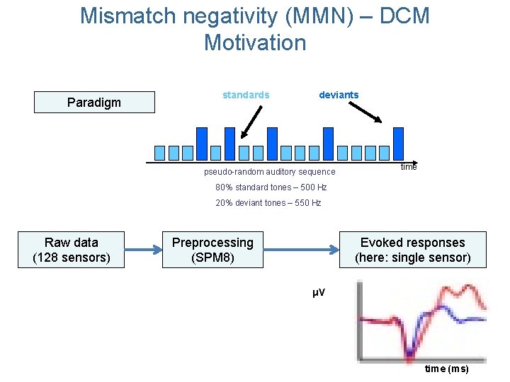
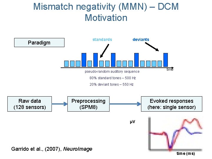
Mismatch negativity (MMN) – DCM Motivation Paradigm standards deviants pseudo-random auditory sequence time 80% standard tones – 500 Hz 20% deviant tones – 550 Hz Raw data (128 sensors) Preprocessing (SPM 8) Evoked responses (here: single sensor) μV time (ms)

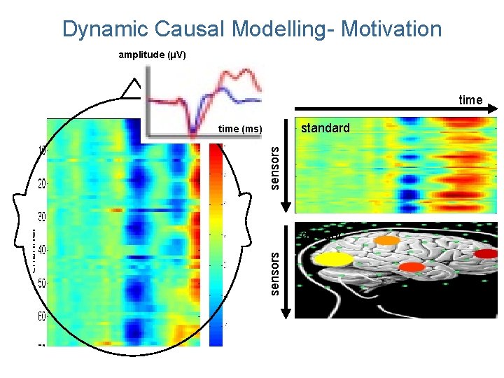
Dynamic Causal Modelling- Motivation amplitude (μV) time standard sensors time (ms) sensors deviant

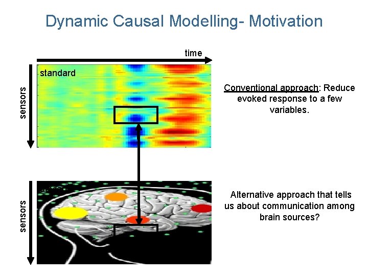
Dynamic Causal Modelling- Motivation time standard sensors Conventional approach: Reduce evoked response to a few variables. sensors deviant Alternative approach that tells us about communication among brain sources?

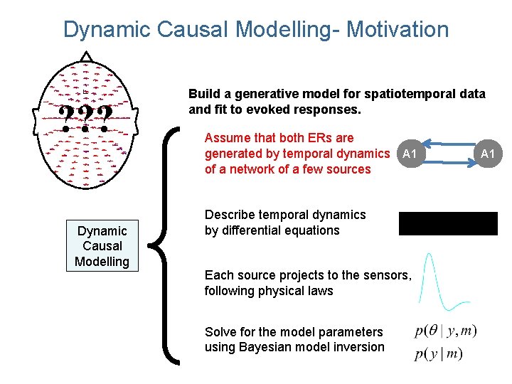
Dynamic Causal Modelling- Motivation ? ? ? Dynamic Causal Modelling Build a generative model for spatiotemporal data and fit to evoked responses. Assume that both ERs are generated by temporal dynamics A 1 of a network of a few sources Describe temporal dynamics by differential equations Each source projects to the sensors, following physical laws Solve for the model parameters using Bayesian model inversion A 1

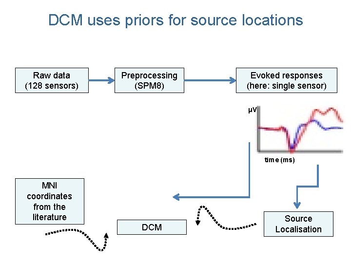
DCM uses priors for source locations Raw data (128 sensors) Preprocessing (SPM 8) Evoked responses (here: single sensor) μV time (ms) MNI coordinates from the literature DCM Source Localisation

Overview Dynamic Causal Modelling – Motivation Dynamic Causal Modelling – Generative model Bayesian model inversion/selection Example

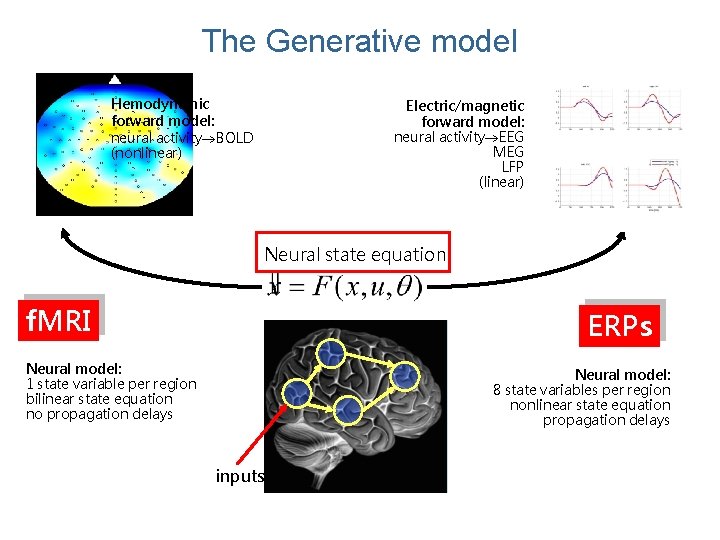
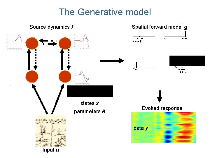
The Generative model Hemodynamic forward model: neural activity BOLD (nonlinear) Electric/magnetic forward model: neural activity EEG MEG LFP (linear) Neural state equation: f. MRI ERPs Neural model: 1 state variable per region bilinear state equation no propagation delays Neural model: 8 state variables per region nonlinear state equation propagation delays inputs

The Generative model Source dynamics f Spatial forward model g states x parameters θ Evoked response data y Input u

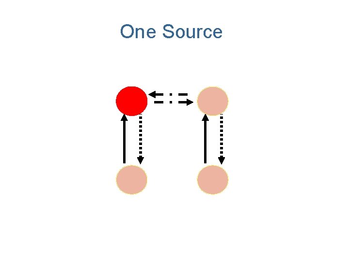
One Source

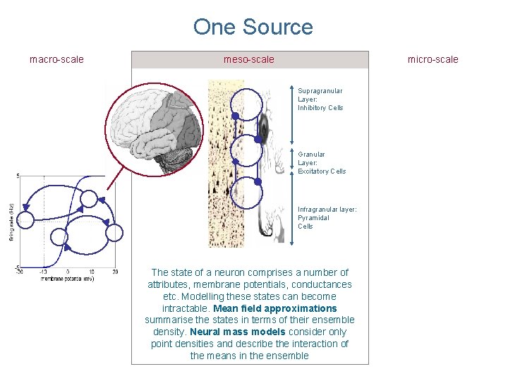
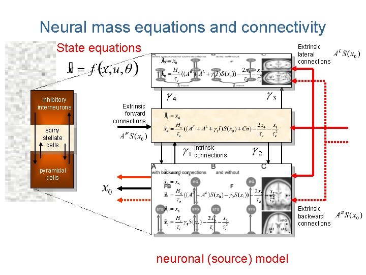
One Source macro-scale meso-scale micro-scale Supragranular Layer: Inhibitory Cells Granular Layer: Excitatory Cells Infragranular layer: Pyramidal Cells The state of a neuron comprises a number of attributes, membrane potentials, conductances etc. Modelling these states can become intractable. Mean field approximations summarise the states in terms of their ensemble density. Neural mass models consider only point densities and describe the interaction of the means in the ensemble

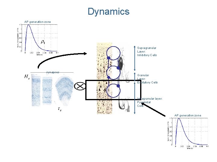
Dynamics AP generation zone Supragranular Layer: Inhibitory Cells synapses Granular Layer: Excitatory Cells Infragranular layer: Pyramidal Cells AP generation zone

Neural mass equations and connectivity State equations inhibitory interneurons spiny stellate cells Extrinsic lateral connections Extrinsic forward connections Intrinsic connections pyramidal cells Extrinsic backward connections neuronal (source) model

Overview Dynamic Causal Modelling – Motivation Dynamic Causal Modelling – Generative model Bayesian model inversion/selection Example

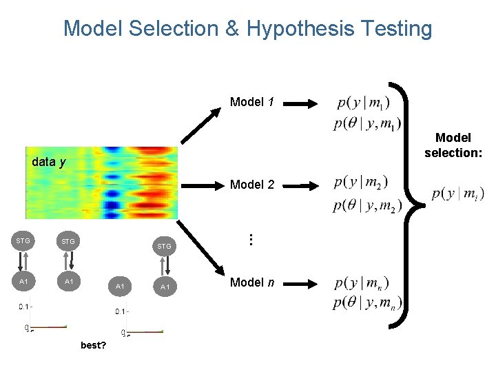
Model Selection & Hypothesis Testing Model 1 Model selection: data y Model 2 STG A 1 best? A 1 . . . STG Model n

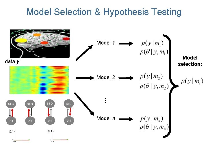
Model Selection & Hypothesis Testing Model 1 Model selection: data y Model 2 STG STG A 1 A 1 . . . STG Model n

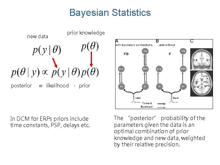
Bayesian Statistics new data posterior prior knowledge likelihood ∙ prior In DCM for ERPs priors include time constants, PSP, delays etc. The “posterior” probability of the parameters given the data is an optimal combination of prior knowledge and new data, weighted by their relative precision.

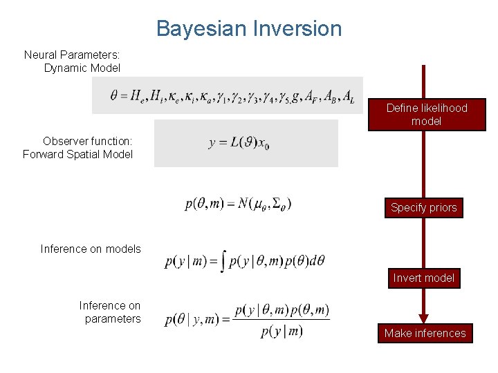
Bayesian Inversion Neural Parameters: Dynamic Model Define likelihood model Observer function: Forward Spatial Model Specify priors Inference on models Invert model Inference on parameters Make inferences

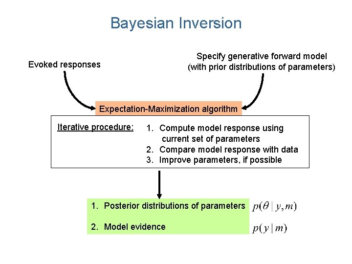
Bayesian Inversion Specify generative forward model (with prior distributions of parameters) Evoked responses Expectation-Maximization algorithm Iterative procedure: 1. Compute model response using current set of parameters 2. Compare model response with data 3. Improve parameters, if possible 1. Posterior distributions of parameters 2. Model evidence

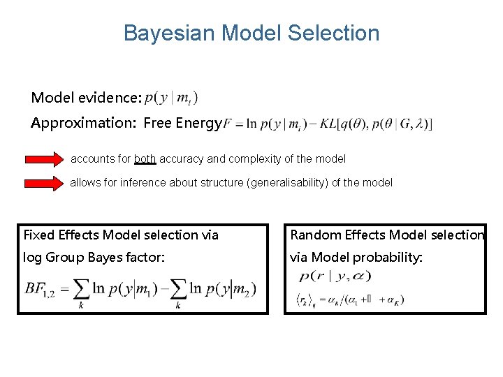
Bayesian Model Selection Model evidence: Approximation: Free Energy accounts for both accuracy and complexity of the model allows for inference about structure (generalisability) of the model Fixed Effects Model selection via Random Effects Model selection log Group Bayes factor: via Model probability:

Overview Dynamic Causal Modelling – Motivation Dynamic Causal Modelling – Generative model Bayesian model inversion/selection Example

Mismatch negativity (MMN) – DCM Motivation standards Paradigm deviants pseudo-random auditory sequence time 80% standard tones – 500 Hz 20% deviant tones – 550 Hz Raw data (128 sensors) Preprocessing (SPM 8) Evoked responses (here: single sensor) μV Garrido et al. , (2007), Neuro. Image time (ms)

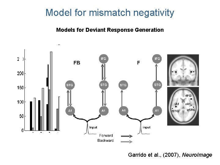
Model for mismatch negativity Models for Deviant Response Generation Garrido et al. , (2007), Neuro. Image

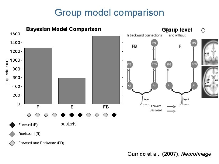
Group model comparison Group level log-evidence Bayesian Model Comparison Forward (F) subjects Backward (B) Forward and Backward (FB) Garrido et al. , (2007), Neuro. Image

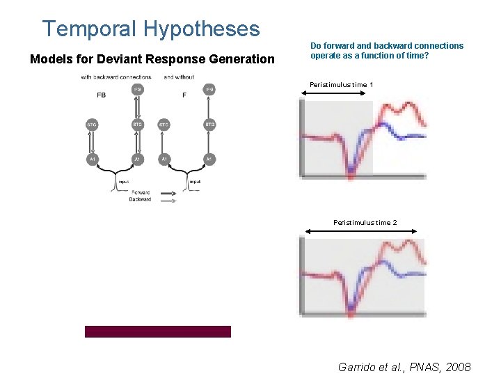
Temporal Hypotheses Models for Deviant Response Generation Do forward and backward connections operate as a function of time? Peristimulus time 1 Peristimulus time 2 Garrido et al. , PNAS, 2008

Grand mean ERPs Garrido M. I. et. al. PNAS 2007; 104: 20961 -20966 © 2007 by National Academy of Sciences

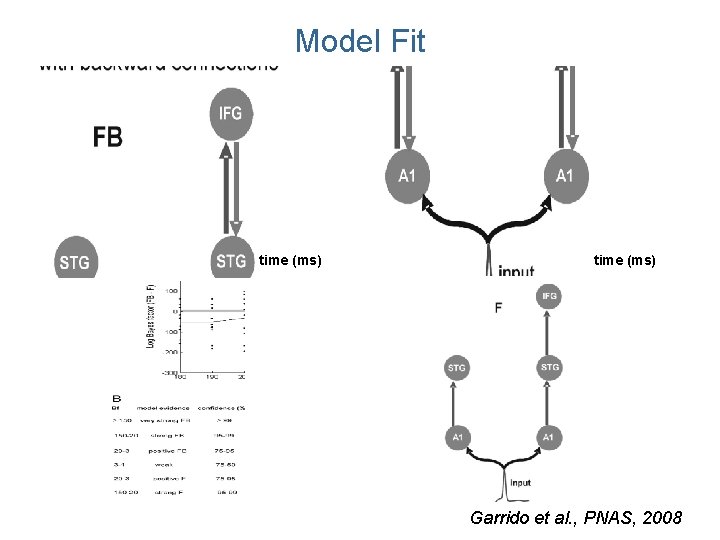
Model Fit time (ms) Garrido et al. , PNAS, 2008

Bayesian model comparison across subjects Garrido M. I. et. al. PNAS 2007; 104: 20961 -20966 © 2007 by National Academy of Sciences

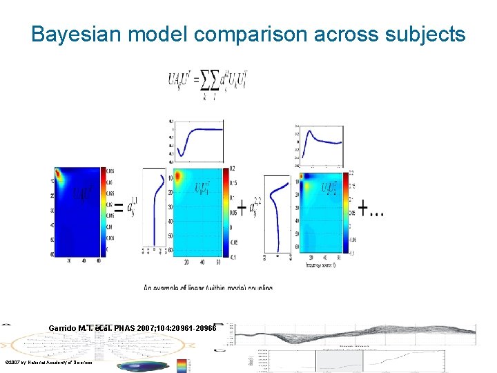
Bayesian model comparison across subjects • First : Forward and Backward Connections are required to produce a deviant, “mismatch” response • Then this was refined to show: Forward Connections are sufficient to generate early components of the mismatch ERP but Forward and Backward connections are required to generate late components of the ERP

Summary DCM enables testing hypotheses about how brain sources communicate. DCM is based on a neurobiologically plausible generative model of evoked responses. Differences between conditions are modelled as modulation of connectivity. Inference: Bayesian model selection Posterior Connectivity Estimates

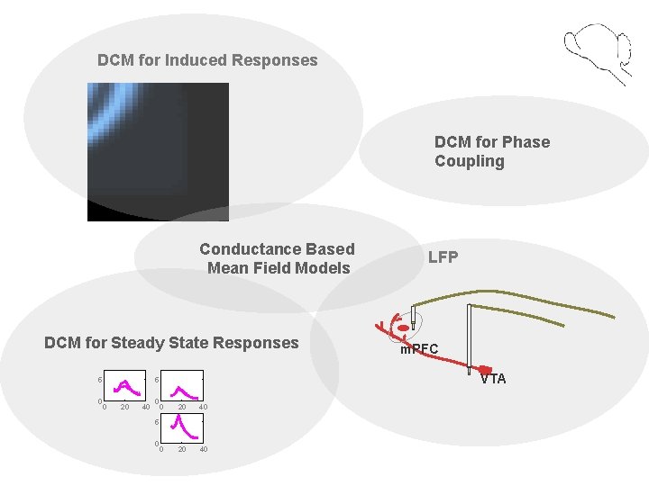
DCM for Induced Responses DCM for Phase Coupling Conductance Based Mean Field Models DCM for Steady State Responses 5 0 20 40 5 0 m. PFC VTA 5 0 LFP