Dual Numbers Simple Math Easy C Coding and

Dual Numbers: Simple Math, Easy C++ Coding, and Lots of Tricks Gino van den Bergen gino@dtecta. com

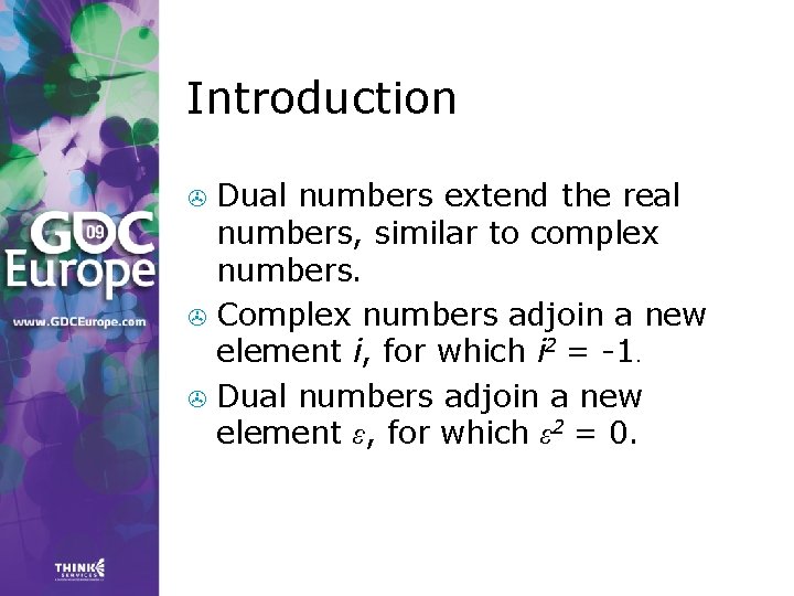
Introduction Dual numbers extend the real numbers, similar to complex numbers. > Complex numbers adjoin a new element i, for which i 2 = -1. > Dual numbers adjoin a new element ε, for which ε 2 = 0. >

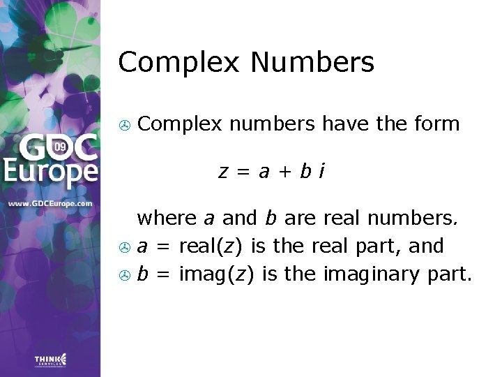
Complex Numbers > Complex numbers have the form z=a+bi where a and b are real numbers. > a = real(z) is the real part, and > b = imag(z) is the imaginary part.

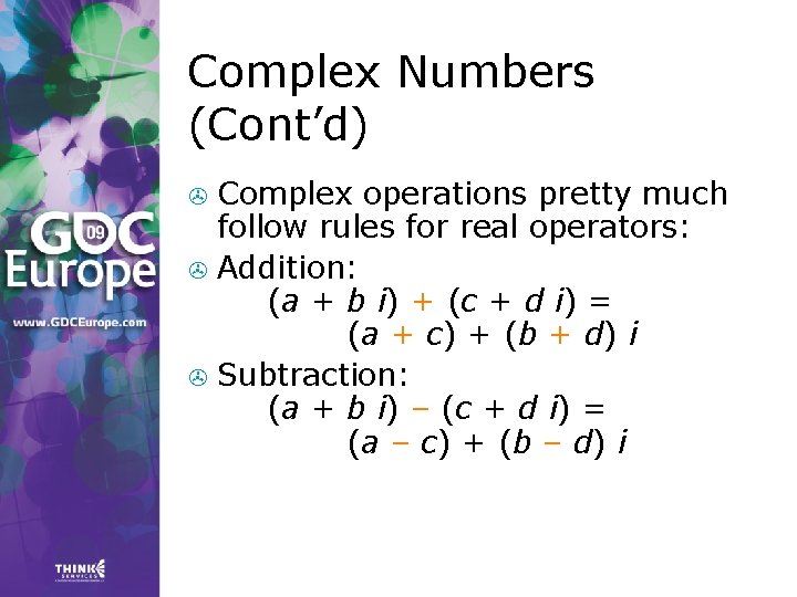
Complex Numbers (Cont’d) Complex operations pretty much follow rules for real operators: > Addition: (a + b i) + (c + d i) = (a + c) + (b + d) i > Subtraction: (a + b i) – (c + d i) = (a – c) + (b – d) i >

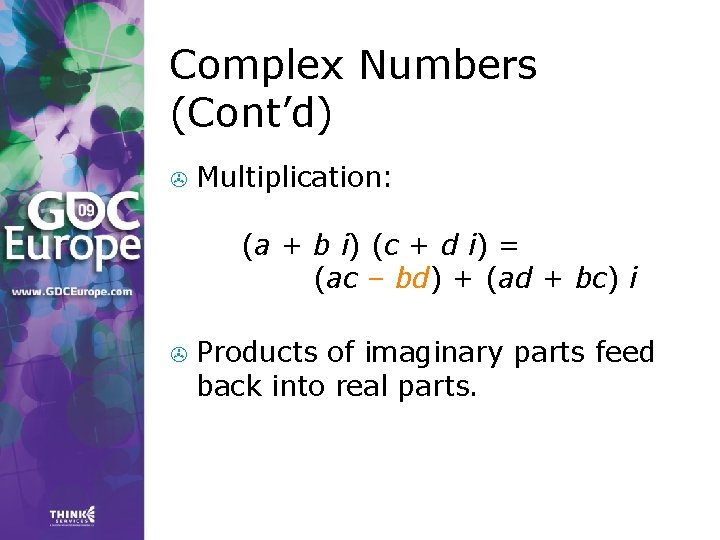
Complex Numbers (Cont’d) > Multiplication: (a + b i) (c + d i) = (ac – bd) + (ad + bc) i > Products of imaginary parts feed back into real parts.

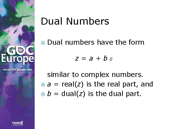
Dual Numbers > Dual numbers have the form z=a+bε similar to complex numbers. > a = real(z) is the real part, and > b = dual(z) is the dual part.

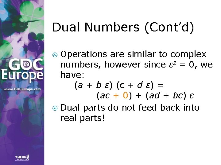
Dual Numbers (Cont’d) Operations are similar to complex numbers, however since ε 2 = 0, we have: (a + b ε) (c + d ε) = (ac + 0) + (ad + bc) ε > Dual parts do not feed back into real parts! >

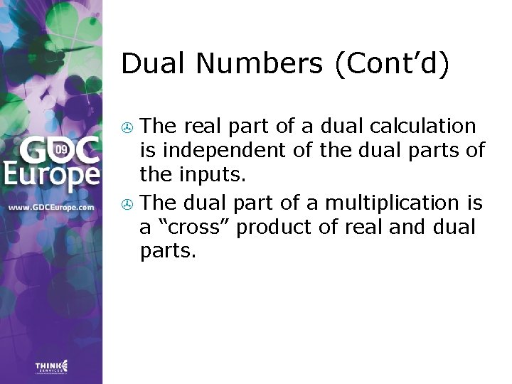
Dual Numbers (Cont’d) The real part of a dual calculation is independent of the dual parts of the inputs. > The dual part of a multiplication is a “cross” product of real and dual parts. >

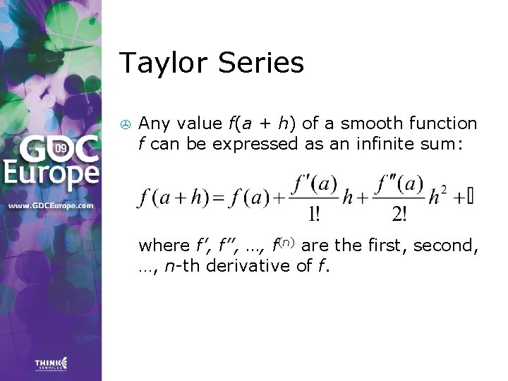
Taylor Series > Any value f(a + h) of a smooth function f can be expressed as an infinite sum: where f’, f’’, …, f(n) are the first, second, …, n-th derivative of f.

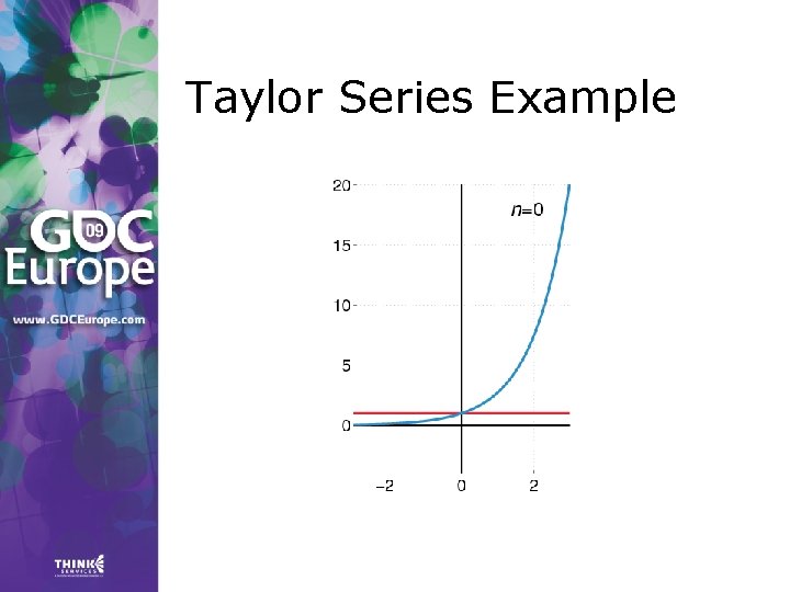
Taylor Series Example

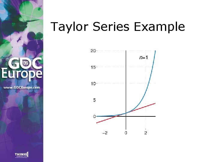
Taylor Series Example

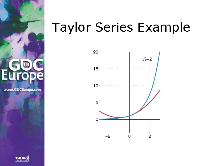
Taylor Series Example

Taylor Series Example

Taylor Series Example

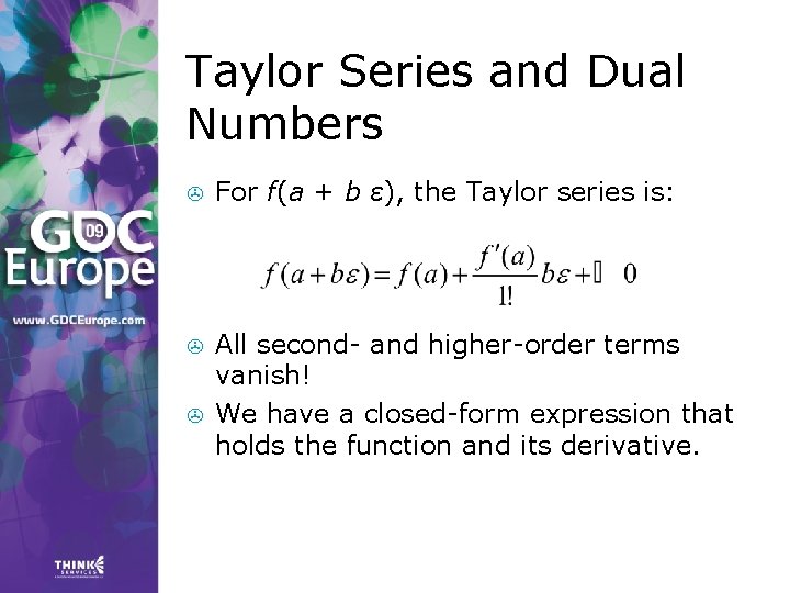
Taylor Series and Dual Numbers > For f(a + b ε), the Taylor series is: > All second- and higher-order terms vanish! We have a closed-form expression that holds the function and its derivative. >

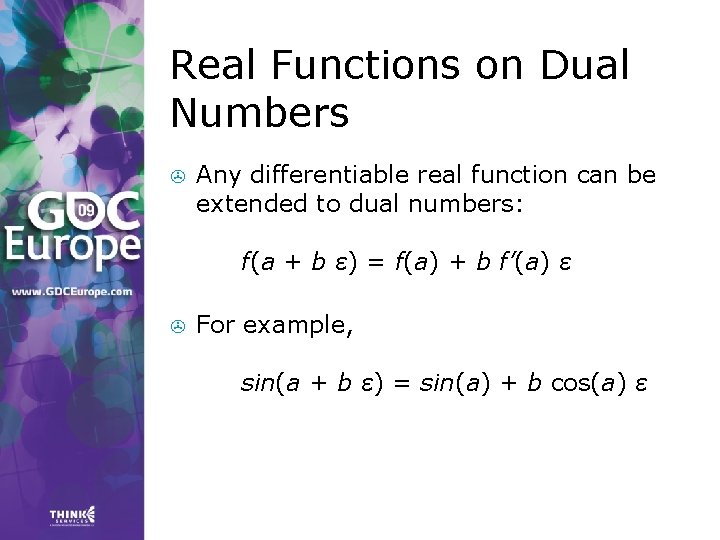
Real Functions on Dual Numbers > Any differentiable real function can be extended to dual numbers: f(a + b ε) = f(a) + b f’(a) ε > For example, sin(a + b ε) = sin(a) + b cos(a) ε

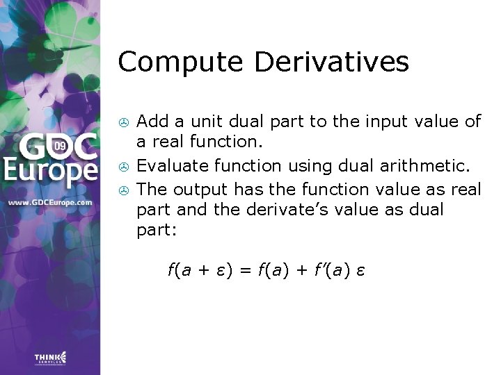
Compute Derivatives > > > Add a unit dual part to the input value of a real function. Evaluate function using dual arithmetic. The output has the function value as real part and the derivate’s value as dual part: f(a + ε) = f(a) + f’(a) ε

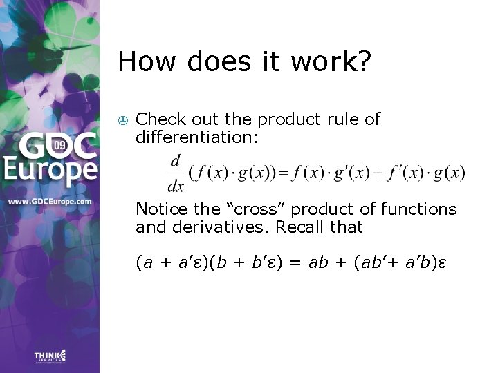
How does it work? > Check out the product rule of differentiation: Notice the “cross” product of functions and derivatives. Recall that (a + a’ε)(b + b’ε) = ab + (ab’+ a’b)ε

Automatic Differentiation in C++ We need some easy way of extending functions on floatingpoint types to dual numbers… > …and we need a type that holds dual numbers and offers operators for performing dual arithmetic. >

Extension by Abstraction > C++ allows you to abstract from the numerical type through: Typedefs > Function templates > Constructors (conversion) > Overloading > Traits class templates >

Abstract Scalar Type > Never use explicit floating-point types, such as float or double. > Instead use a type name, e. g. Scalar, either as template parameter or as typedef: typedef float Scalar;

Constructors > Primitive types have constructors as well: Default: float() == 0. 0 f > Conversion: float(2) == 2. 0 f > > Use constructors for defining constants, e. g. use Scalar(2), rather than 2. 0 f or (Scalar)2.

Overloading > > Operators and functions on primitive types can be overloaded in hand-baked classes, e. g. std: : complex. Primitive types use operators: +, -, *, / …and functions: sqrt, pow, sin, … NB: Use <cmath> rather than <math. h>. That is, use sqrt NOT sqrtf on floats.

Traits Class Templates > Type-dependent constants, e. g. machine epsilon, are obtained through a traits class defined in <limits>. > Use std: : numeric_limits<T>: : epsilon() rather than FLT_EPSILON. > Either specialize this traits template for hand-baked classes or create your own traits class template.

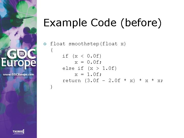
Example Code (before) > float smoothstep(float x) { if (x < 0. 0 f) x = 0. 0 f; else if (x > 1. 0 f) x = 1. 0 f; return (3. 0 f – 2. 0 f * x) * x; }

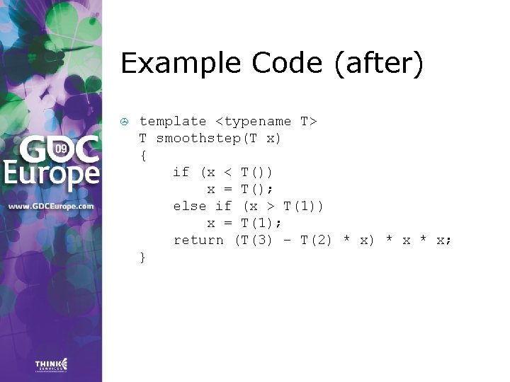
Example Code (after) > template <typename T> T smoothstep(T x) { if (x < T()) x = T(); else if (x > T(1)) x = T(1); return (T(3) – T(2) * x * x; }

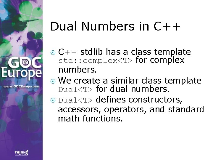
Dual Numbers in C++ stdlib has a class template std: : complex<T> for complex numbers. > We create a similar class template Dual<T> for dual numbers. > Dual<T> defines constructors, accessors, operators, and standard math functions. >

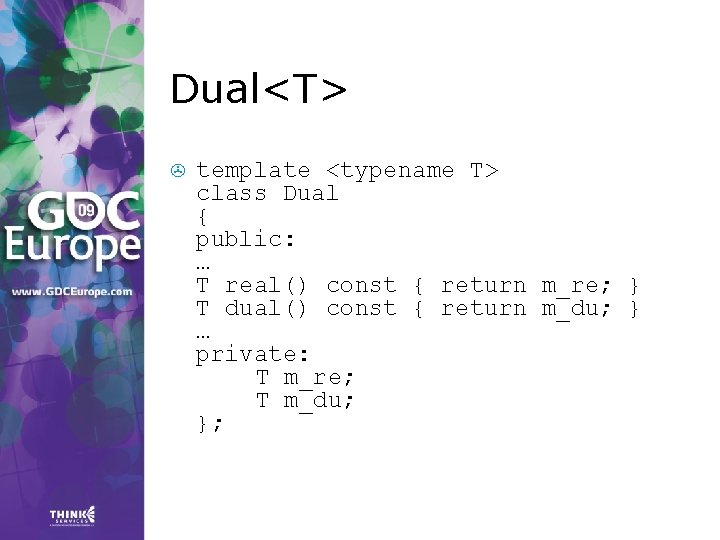
Dual<T> > template <typename T> class Dual { public: … T real() const { return m_re; } T dual() const { return m_du; } … private: T m_re; T m_du; };

Dual<T>: Constructor > template <typename T> Dual<T>: : Dual(T re = T(), T du = T()) : m_re(re) , m_du(du) {} … Dual<float> z 1; // zero initialized Dual<float> z 2(2); // zero dual part Dual<float> z 3(2, 1);

Dual<T>: operators > template <typename T> Dual<T> operator*(Dual<T> a, Dual<T> b) { return Dual<T>( a. real() * b. real(), a. real() * b. dual() + a. dual() * b. real() ); }

Dual<T>: operators (Cont’d) > We also need these template <typename T> Dual<T> operator*(Dual<T> a, T b); template <typename T> Dual<T> operator*(T a, Dual<T> b); since template argument deduction does not perform implicit type conversions.

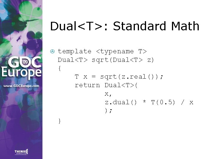
Dual<T>: Standard Math > template <typename T> Dual<T> sqrt(Dual<T> z) { T x = sqrt(z. real()); return Dual<T>( x, z. dual() * T(0. 5) / x ); }

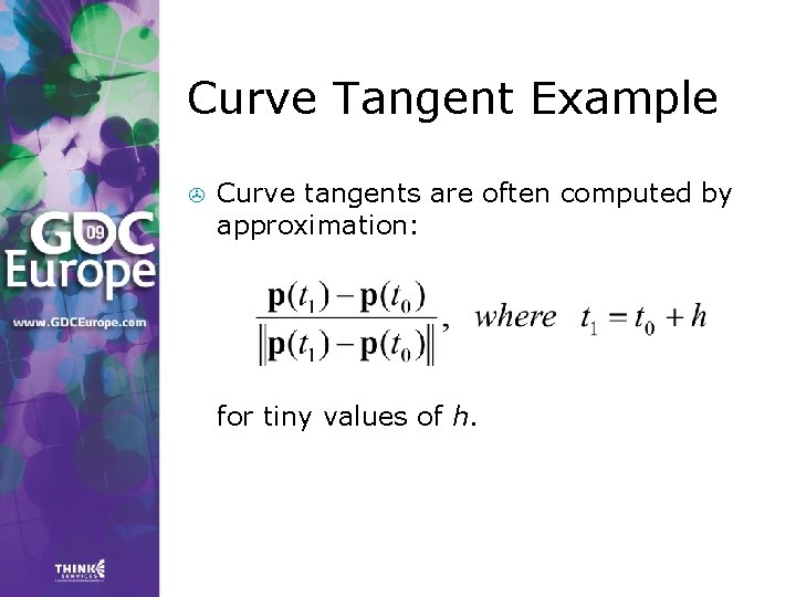
Curve Tangent Example > Curve tangents are often computed by approximation: for tiny values of h.

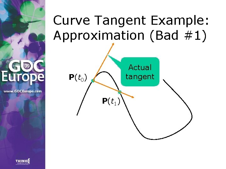
Curve Tangent Example: Approximation (Bad #1) Actual tangent P(t 0) P(t 1)

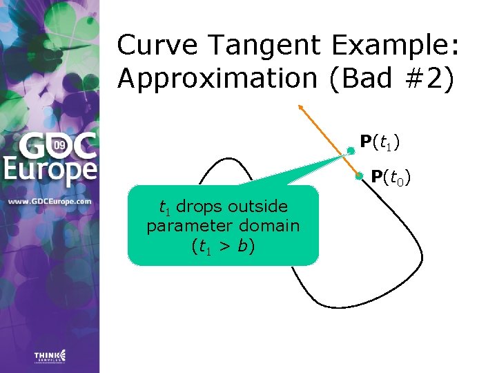
Curve Tangent Example: Approximation (Bad #2) P(t 1) P(t 0) t 1 drops outside parameter domain (t 1 > b)

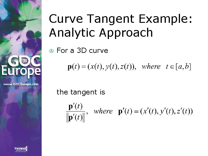
Curve Tangent Example: Analytic Approach > For a 3 D curve the tangent is

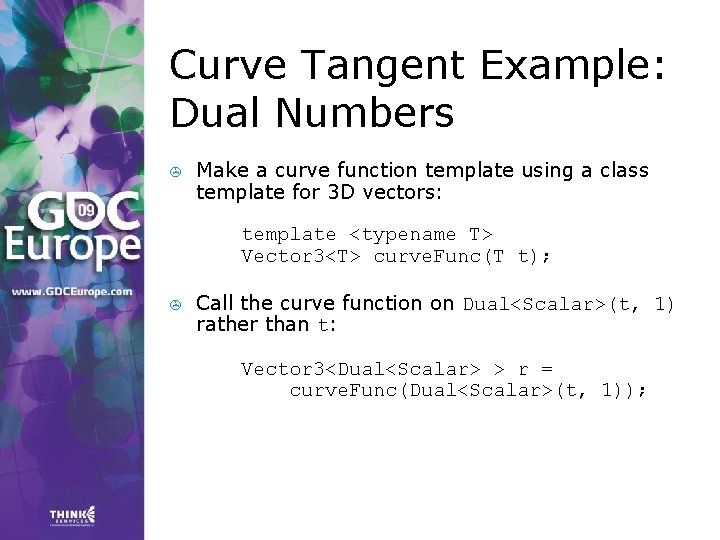
Curve Tangent Example: Dual Numbers > Make a curve function template using a class template for 3 D vectors: template <typename T> Vector 3<T> curve. Func(T t); > Call the curve function on Dual<Scalar>(t, 1) rather than t: Vector 3<Dual<Scalar> > r = curve. Func(Dual<Scalar>(t, 1));

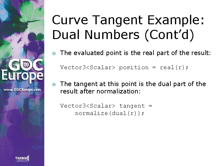
Curve Tangent Example: Dual Numbers (Cont’d) > The evaluated point is the real part of the result: Vector 3<Scalar> position = real(r); > The tangent at this point is the dual part of the result after normalization: Vector 3<Scalar> tangent = normalize(dual(r));

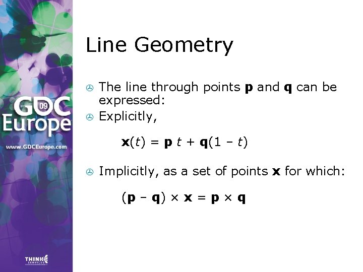
Line Geometry > > The line through points p and q can be expressed: Explicitly, x(t) = p t + q(1 – t) > Implicitly, as a set of points x for which: (p – q) × x = p × q

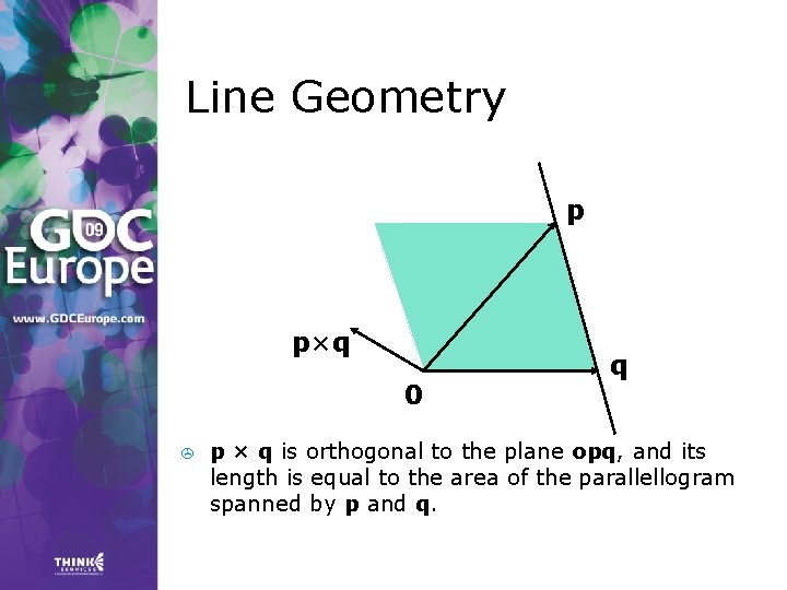
Line Geometry p p×q 0 > q p × q is orthogonal to the plane opq, and its length is equal to the area of the parallellogram spanned by p and q.

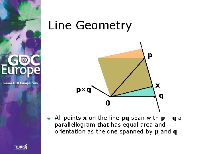
Line Geometry p x p×q 0 > q All points x on the line pq span with p – q a parallellogram that has equal area and orientation as the one spanned by p and q.

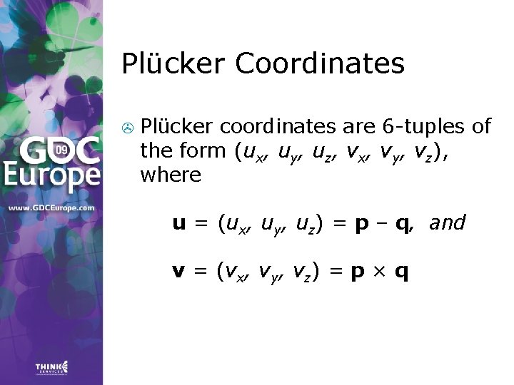
Plücker Coordinates > Plücker coordinates are 6 -tuples of the form (ux, uy, uz, vx, vy, vz), where u = (ux, uy, uz) = p – q, and v = (vx, vy, vz) = p × q

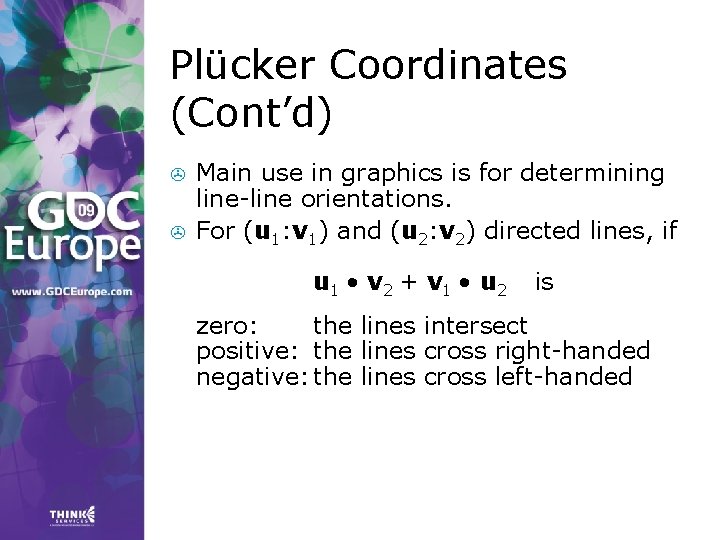
Plücker Coordinates (Cont’d) > > Main use in graphics is for determining line-line orientations. For (u 1: v 1) and (u 2: v 2) directed lines, if u 1 • v 2 + v 1 • u 2 is zero: the lines intersect positive: the lines cross right-handed negative: the lines cross left-handed

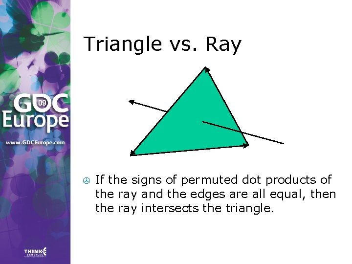
Triangle vs. Ray > If the signs of permuted dot products of the ray and the edges are all equal, then the ray intersects the triangle.

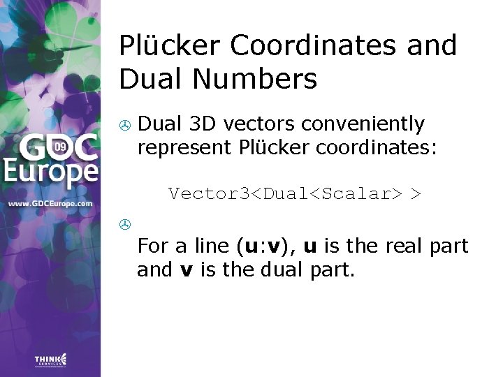
Plücker Coordinates and Dual Numbers > Dual 3 D vectors conveniently represent Plücker coordinates: Vector 3<Dual<Scalar> > > For a line (u: v), u is the real part and v is the dual part.

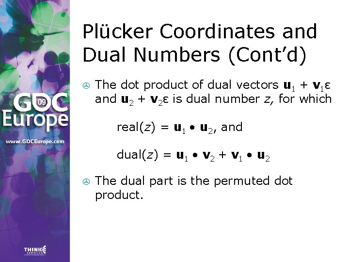
Plücker Coordinates and Dual Numbers (Cont’d) > The dot product of dual vectors u 1 + v 1ε and u 2 + v 2ε is dual number z, for which real(z) = u 1 • u 2, and dual(z) = u 1 • v 2 + v 1 • u 2 > The dual part is the permuted dot product.

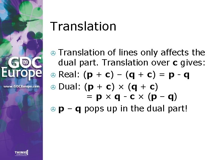
Translation of lines only affects the dual part. Translation over c gives: > Real: (p + c) – (q + c) = p - q > Dual: (p + c) × (q + c) = p × q - c × (p – q) > p – q pops up in the dual part! >

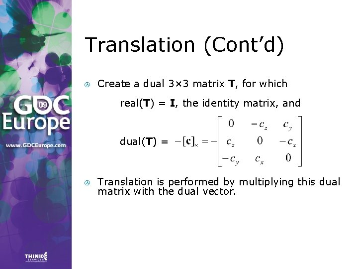
Translation (Cont’d) > Create a dual 3× 3 matrix T, for which real(T) = I, the identity matrix, and dual(T) = > Translation is performed by multiplying this dual matrix with the dual vector.

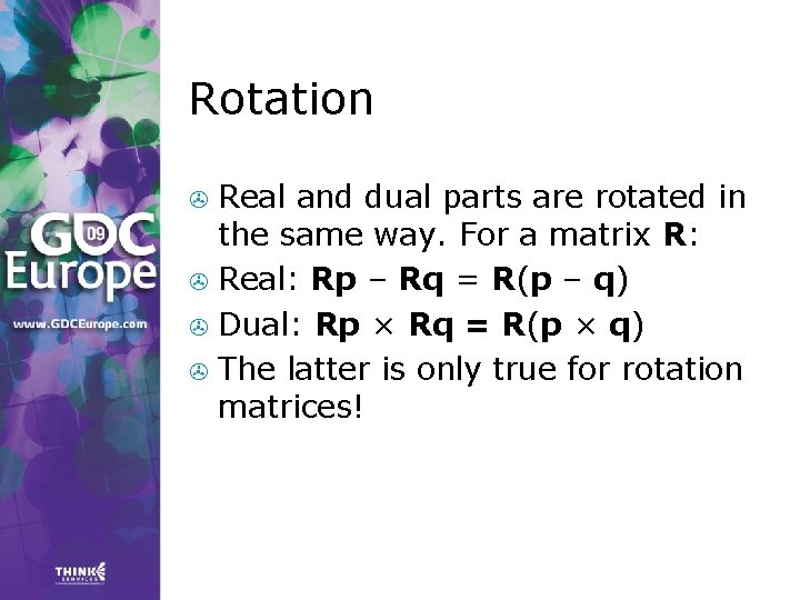
Rotation Real and dual parts are rotated in the same way. For a matrix R: > Real: Rp – Rq = R(p – q) > Dual: Rp × Rq = R(p × q) > The latter is only true for rotation matrices! >

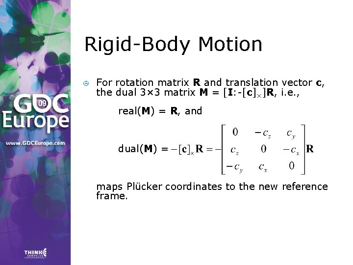
Rigid-Body Motion > For rotation matrix R and translation vector c, the dual 3× 3 matrix M = [I: -[c]×]R, i. e. , real(M) = R, and dual(M) = maps Plücker coordinates to the new reference frame.

Further Reading > > > Motor Algebra: Linear and angular velocity of a rigid body combined in a dual 3 D vector. Screw Theory: Any rigid motion can be expressed as a screw motion, which is represented by a dual quaternion. Spatial Vector Algebra: Featherstone uses 6 D vectors for representing velocities and forces in robot dynamics.

References > > D. Vandevoorde and N. M. Josuttis. C++ Templates: The Complete Guide. Addison. Wesley, 2003. K. Shoemake. Plücker Coordinate Tutorial. Ray Tracing News, Vol. 11, No. 1 R. Featherstone. Robot Dynamics Algorithms. Kluwer Academic Publishers, 1987. L. Kavan et al. Skinning with dual quaternions. Proc. ACM SIGGRAPH Symposium on Interactive 3 D Graphics and Games, 2007

Conclusions Abstract from numerical types in your C++ code. > Differentiation is easy, fast, and accurate with dual numbers. > Dual numbers have other uses as well. Explore yourself! >

Thank You! > Check out sample code soon to be released on: http: //www. dtecta. com