DSPCIS PartII Filter Design Implementation Chapter4 Filter Design

DSP-CIS Part-II : Filter Design & Implementation Chapter-4 : Filter Design Marc Moonen Dept. E. E. /ESAT-STADIUS, KU Leuven marc. moonen@kuleuven. be www. esat. kuleuven. be/stadius/

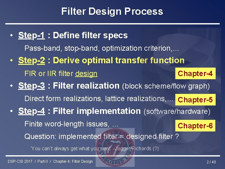
Filter Design Process • Step-1 : Define filter specs Pass-band, stop-band, optimization criterion, … • Step-2 : Derive optimal transfer function FIR or IIR filter design Chapter-4 • Step-3 : Filter realization (block scheme/flow graph) Direct form realizations, lattice realizations, … Chapter-5 • Step-4 : Filter implementation (software/hardware) Finite word-length issues, … Chapter-6 Question: implemented filter = designed filter ? ‘You can’t always get what you want’ -Jagger/Richards (? ) DSP-CIS 2017 / Part-II / Chapter-4: Filter Design 2 / 40

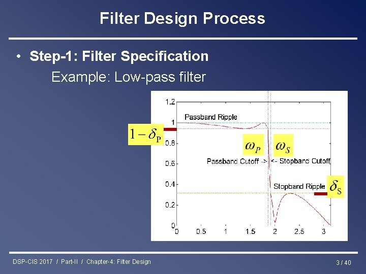
Filter Design Process • Step-1: Filter Specification Example: Low-pass filter DSP-CIS 2017 / Part-II / Chapter-4: Filter Design 3 / 40

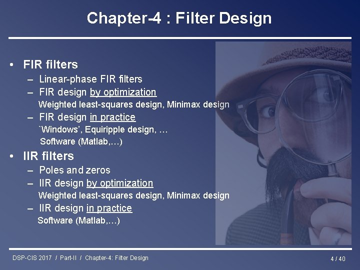
Chapter-4 : Filter Design • FIR filters – Linear-phase FIR filters – FIR design by optimization Weighted least-squares design, Minimax design – FIR design in practice `Windows’, Equiripple design, … Software (Matlab, …) • IIR filters – Poles and zeros – IIR design by optimization Weighted least-squares design, Minimax design – IIR design in practice Software (Matlab, …) DSP-CIS 2017 / Part-II / Chapter-4: Filter Design 4 / 40

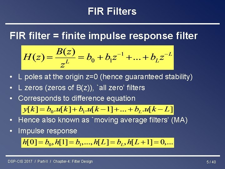
FIR Filters FIR filter = finite impulse response filter • L poles at the origin z=0 (hence guaranteed stability) • L zeros (zeros of B(z)), `all zero’ filters • Corresponds to difference equation • Hence also known as `moving average filters’ (MA) • Impulse response DSP-CIS 2017 / Part-II / Chapter-4: Filter Design 5 / 40

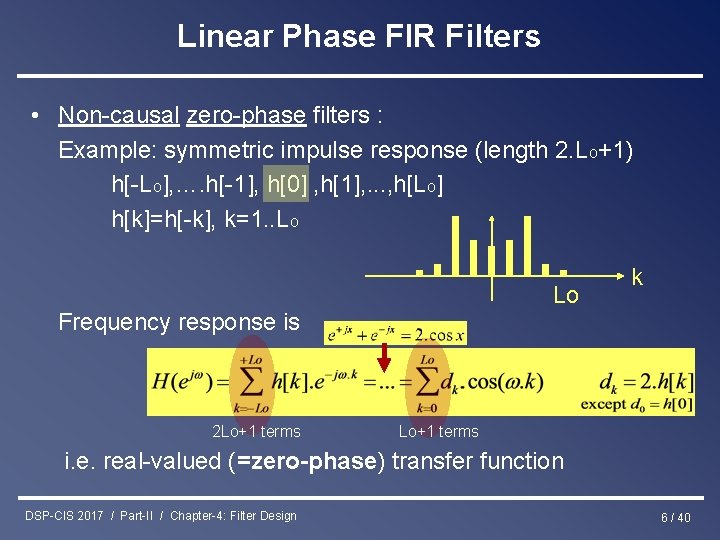
Linear Phase FIR Filters • Non-causal zero-phase filters : Example: symmetric impulse response (length 2. Lo+1) h[-Lo], …. h[-1], h[0] , h[1], . . . , h[Lo] h[k]=h[-k], k=1. . Lo Lo k Frequency response is 2 Lo+1 terms i. e. real-valued (=zero-phase) transfer function DSP-CIS 2017 / Part-II / Chapter-4: Filter Design 6 / 40

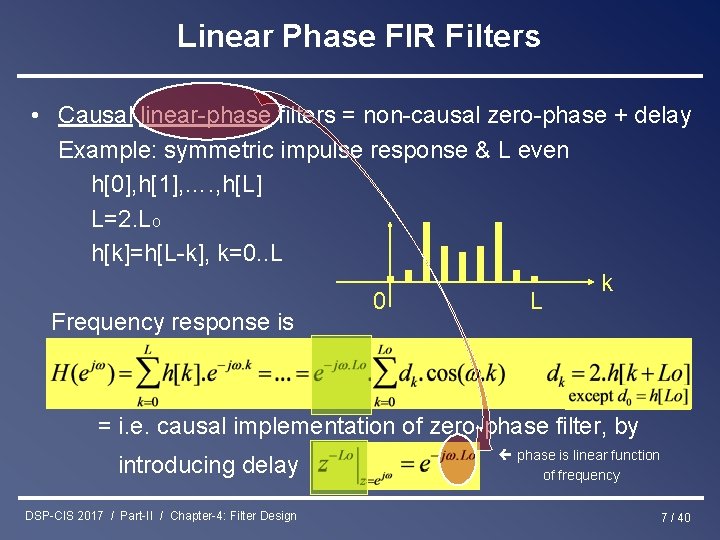
Linear Phase FIR Filters • Causal linear-phase filters = non-causal zero-phase + delay Example: symmetric impulse response & L even h[0], h[1], …. , h[L] L=2. Lo h[k]=h[L-k], k=0. . L k 0 L Frequency response is = i. e. causal implementation of zero-phase filter, by introducing delay DSP-CIS 2017 / Part-II / Chapter-4: Filter Design phase is linear function of frequency 7 / 40

Linear Phase FIR Filters Type-1 L=2 Lo=even symmetric h[k]=h[L-k] Type-2 L=2 Lo+1=odd h[k]=h[L-k] h[k]=-h[L-k] LP/HP/BP zero at LP/BP zero at HP/BP symmetric Type-3 L=2 Lo=even anti-symmetric Type-4 L=2 Lo+1=odd anti-symmetric PS: `Modulating’ Type-2 with 1, -1, . . gives Type-4 (LP->HP) PS: `Modulating’ Type-4 with 1, -1, . . gives Type-2 (HP->LP) PS: `Modulating’ Type-1 with 1, -1, . . gives Type-1 (LP<->HP) PS: `Modulating’ Type-3 with 1, -1, . . gives Type-3 (BP<->BP) PS: IIR filters can NEVER have linear-phase property ! (proof see literature) DSP-CIS 2017 / Part-II / Chapter-4: Filter Design 8 / 40

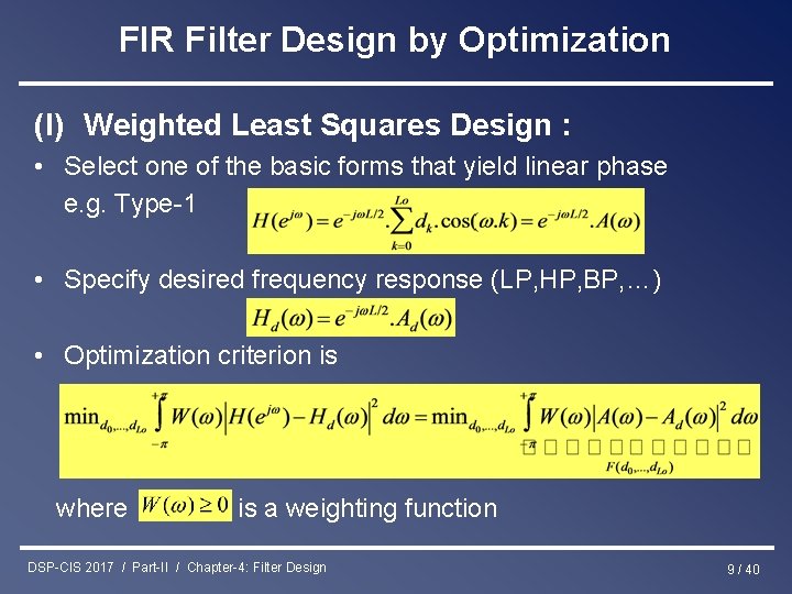
FIR Filter Design by Optimization (I) Weighted Least Squares Design : • Select one of the basic forms that yield linear phase e. g. Type-1 • Specify desired frequency response (LP, HP, BP, …) • Optimization criterion is where is a weighting function DSP-CIS 2017 / Part-II / Chapter-4: Filter Design 9 / 40

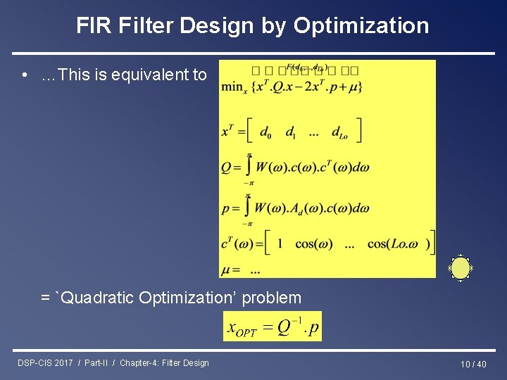
FIR Filter Design by Optimization • …This is equivalent to = `Quadratic Optimization’ problem DSP-CIS 2017 / Part-II / Chapter-4: Filter Design 10 / 40

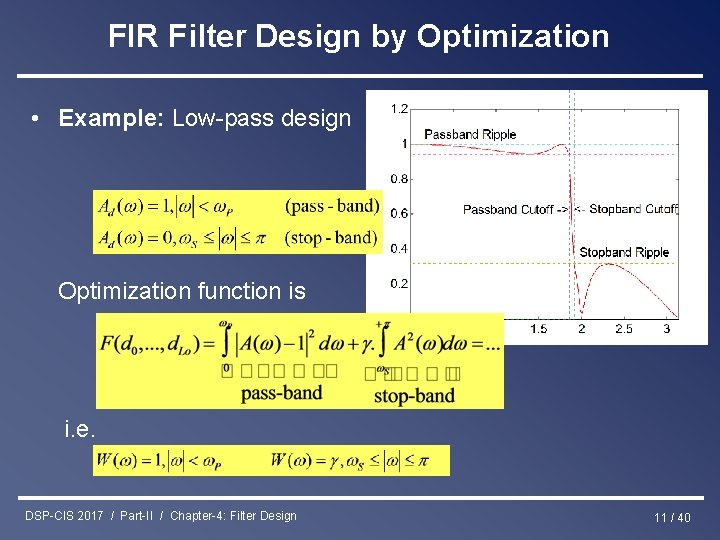
FIR Filter Design by Optimization • Example: Low-pass design Optimization function is i. e. DSP-CIS 2017 / Part-II / Chapter-4: Filter Design 11 / 40

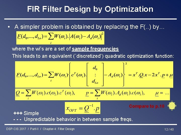
FIR Filter Design by Optimization • A simpler problem is obtained by replacing the F(. . ) by… where the wi’s are a set of sample frequencies This leads to an equivalent (`discretized’) quadratic optimization function: Compare to p. 10 +++ Simple - - - Unpredictable behavior in between sample freqs. DSP-CIS 2017 / Part-II / Chapter-4: Filter Design 12 / 40

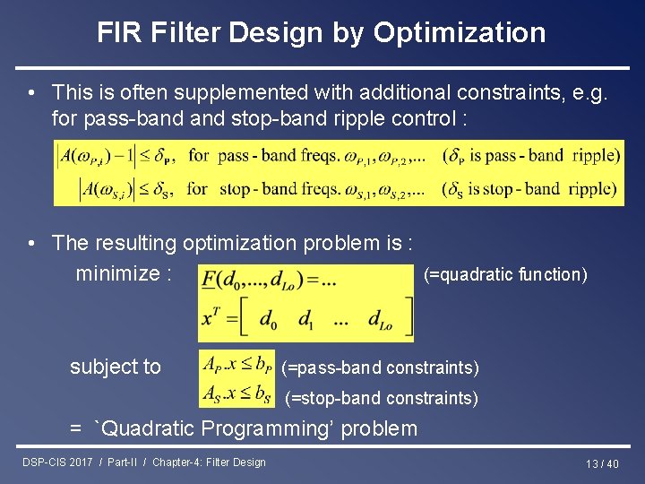
FIR Filter Design by Optimization • This is often supplemented with additional constraints, e. g. for pass-band stop-band ripple control : • The resulting optimization problem is : minimize : (=quadratic function) subject to (=pass-band constraints) (=stop-band constraints) = `Quadratic Programming’ problem DSP-CIS 2017 / Part-II / Chapter-4: Filter Design 13 / 40

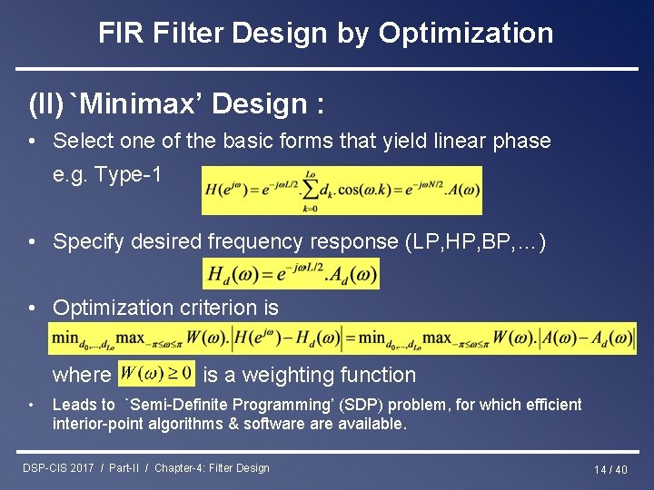
FIR Filter Design by Optimization (II) `Minimax’ Design : • Select one of the basic forms that yield linear phase e. g. Type-1 • Specify desired frequency response (LP, HP, BP, …) • Optimization criterion is where • is a weighting function Leads to `Semi-Definite Programming’ (SDP) problem, for which efficient interior-point algorithms & software available. DSP-CIS 2017 / Part-II / Chapter-4: Filter Design 14 / 40

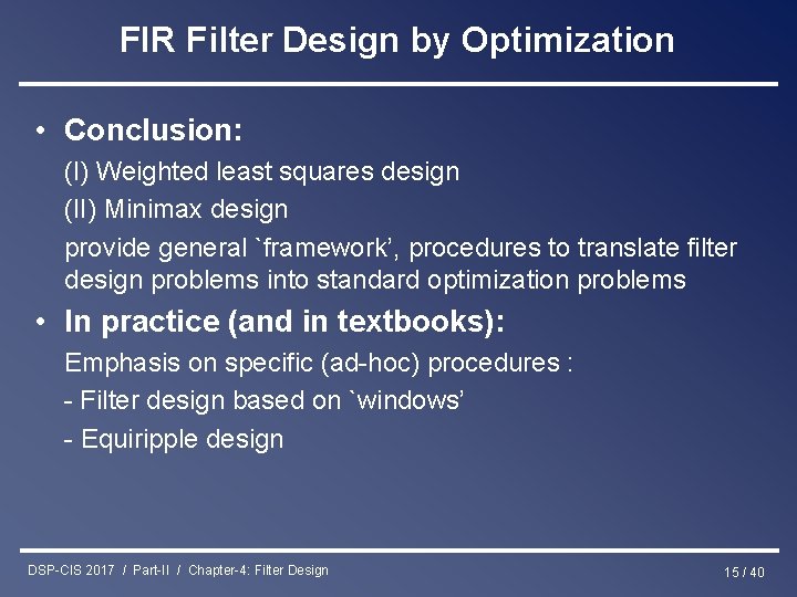
FIR Filter Design by Optimization • Conclusion: (I) Weighted least squares design (II) Minimax design provide general `framework’, procedures to translate filter design problems into standard optimization problems • In practice (and in textbooks): Emphasis on specific (ad-hoc) procedures : - Filter design based on `windows’ - Equiripple design DSP-CIS 2017 / Part-II / Chapter-4: Filter Design 15 / 40

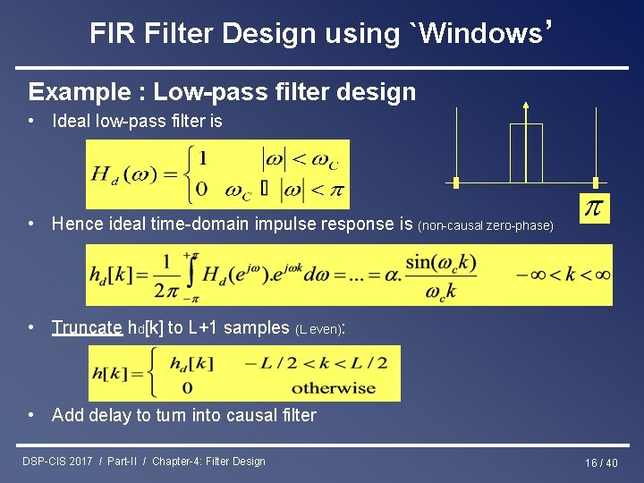
FIR Filter Design using `Windows’ Example : Low-pass filter design • Ideal low-pass filter is • Hence ideal time-domain impulse response is (non-causal zero-phase) • Truncate hd[k] to L+1 samples (L even): • Add delay to turn into causal filter DSP-CIS 2017 / Part-II / Chapter-4: Filter Design 16 / 40

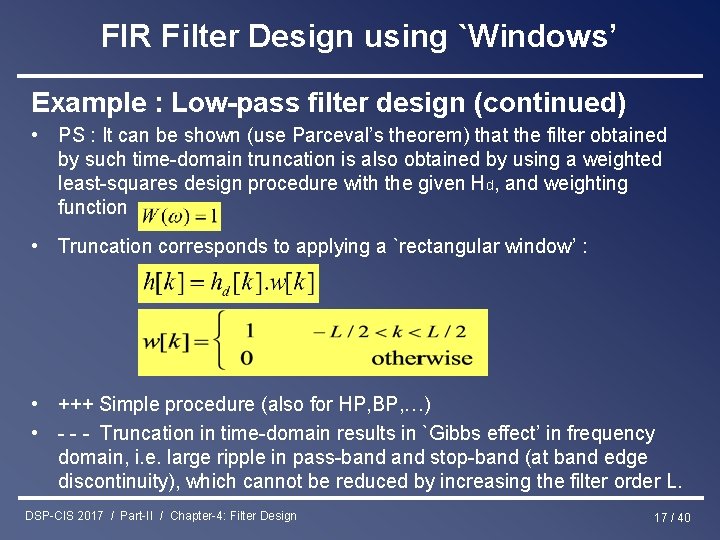
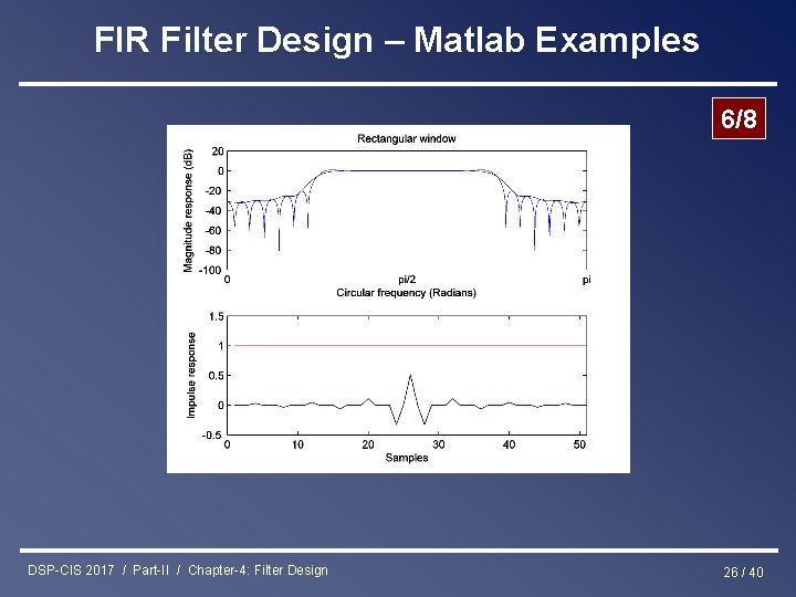
FIR Filter Design using `Windows’ Example : Low-pass filter design (continued) • PS : It can be shown (use Parceval’s theorem) that the filter obtained by such time-domain truncation is also obtained by using a weighted least-squares design procedure with the given Hd, and weighting function • Truncation corresponds to applying a `rectangular window’ : • +++ Simple procedure (also for HP, BP, …) • - - - Truncation in time-domain results in `Gibbs effect’ in frequency domain, i. e. large ripple in pass-band stop-band (at band edge discontinuity), which cannot be reduced by increasing the filter order L. DSP-CIS 2017 / Part-II / Chapter-4: Filter Design 17 / 40

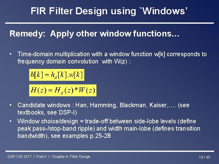
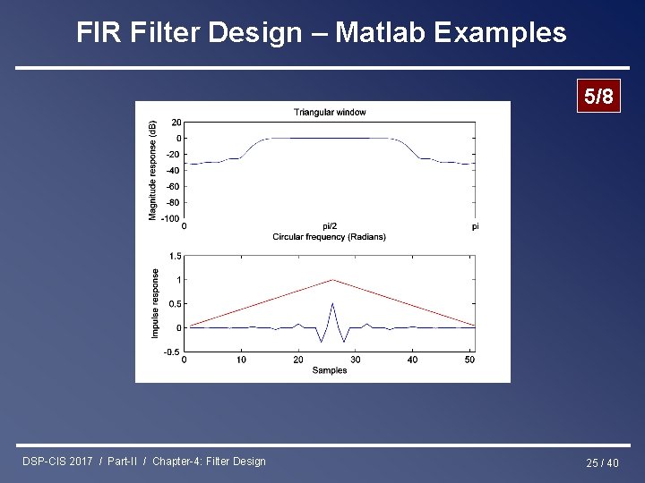
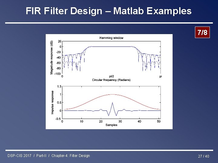
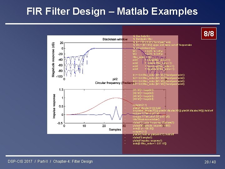
FIR Filter Design using `Windows’ Remedy: Apply other window functions… • Time-domain multiplication with a window function w[k] corresponds to frequency domain convolution with W(z) : • Candidate windows : Han, Hamming, Blackman, Kaiser, …. (see textbooks, see DSP-I) • Window choice/design = trade-off between side-lobe levels (define peak pass-/stop-band ripple) and width main-lobe (defines transition bandwidth), see examples p. 25 -28 DSP-CIS 2017 / Part-II / Chapter-4: Filter Design 18 / 40

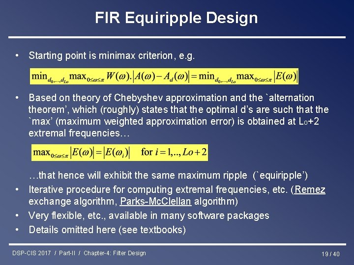
FIR Equiripple Design • Starting point is minimax criterion, e. g. • Based on theory of Chebyshev approximation and the `alternation theorem’, which (roughly) states that the optimal d’s are such that the `max’ (maximum weighted approximation error) is obtained at Lo+2 extremal frequencies… …that hence will exhibit the same maximum ripple (`equiripple’) • Iterative procedure for computing extremal frequencies, etc. (Remez exchange algorithm, Parks-Mc. Clellan algorithm) • Very flexible, etc. , available in many software packages • Details omitted here (see textbooks) DSP-CIS 2017 / Part-II / Chapter-4: Filter Design 19 / 40

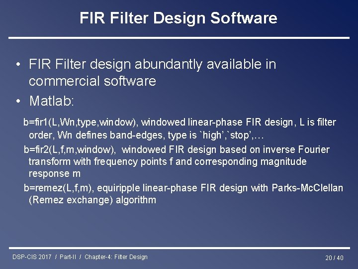
FIR Filter Design Software • FIR Filter design abundantly available in commercial software • Matlab: b=fir 1(L, Wn, type, window), windowed linear-phase FIR design, L is filter order, Wn defines band-edges, type is `high’, `stop’, … b=fir 2(L, f, m, window), windowed FIR design based on inverse Fourier transform with frequency points f and corresponding magnitude response m b=remez(L, f, m), equiripple linear-phase FIR design with Parks-Mc. Clellan (Remez exchange) algorithm DSP-CIS 2017 / Part-II / Chapter-4: Filter Design 20 / 40

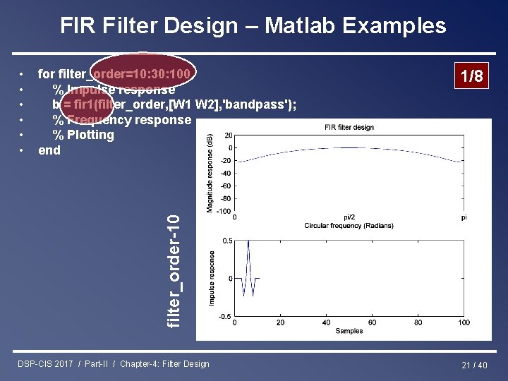
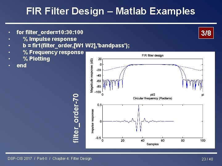
FIR Filter Design – Matlab Examples for filter_order=10: 30: 100 % Impulse response b = fir 1(filter_order, [W 1 W 2], 'bandpass'); % Frequency response % Plotting end 1/8 filter_order-10 • • • DSP-CIS 2017 / Part-II / Chapter-4: Filter Design 21 / 40

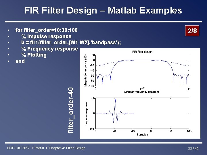
FIR Filter Design – Matlab Examples for filter_order=10: 30: 100 % Impulse response b = fir 1(filter_order, [W 1 W 2], 'bandpass'); % Frequency response % Plotting end 2/8 filter_order-40 • • • DSP-CIS 2017 / Part-II / Chapter-4: Filter Design 22 / 40

FIR Filter Design – Matlab Examples for filter_order=10: 30: 100 % Impulse response b = fir 1(filter_order, [W 1 W 2], 'bandpass'); % Frequency response % Plotting end 3/8 filter_order-70 • • • DSP-CIS 2017 / Part-II / Chapter-4: Filter Design 23 / 40

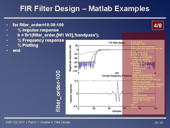
FIR Filter Design – Matlab Examples for filter_order=10: 30: 100 % Impulse response b = fir 1(filter_order, [W 1 W 2], 'bandpass'); % Frequency response % Plotting end filter_order-100 • • • DSP-CIS 2017 / Part-II / Chapter-4: Filter Design 4/8 • • • • • • • % See help fir 1 % Bandpass filter % B = FIR 1(N, Wn, 'bandpass') % Wn = [W 1 W 2] upper and lower cutoff freq W 1 = 0. 25; % 1/4*pi W 2 = 0. 75; % 3/4*pi for filter_order=10: 30: 100 % Impulse response b = fir 1(filter_order, [W 1 W 2], 'bandpass'); % Frequency response [H W]=freqz(b); % Plotting subplot(211) plot(W, db(abs(H))); hold on set(gca, 'XTick', 0: pi/2: pi) set(gca, 'XTick. Label', {'0', 'pi/2', 'pi'}) title('FIR filter design'); xlabel('Circular frequency (Radians)'); ylabel('Magnitude response (d. B)'); axis([0 pi -100 20]) subplot(212) plot(b) xlabel('Samples'); ylabel('Impulse response'); axis([0 100 -0. 5]) pause end hold off 24 / 40

FIR Filter Design – Matlab Examples 5/8 DSP-CIS 2017 / Part-II / Chapter-4: Filter Design 25 / 40

FIR Filter Design – Matlab Examples 6/8 DSP-CIS 2017 / Part-II / Chapter-4: Filter Design 26 / 40

FIR Filter Design – Matlab Examples 7/8 DSP-CIS 2017 / Part-II / Chapter-4: Filter Design 27 / 40

FIR Filter Design – Matlab Examples • • • • • • • • • DSP-CIS 2017 / Part-II / Chapter-4: Filter Design % See help fir 1 % Bandpass filter % B = FIR 1(N, Wn, 'bandpass', win) % Wn = [W 1 W 2] upper and lower cut-off frequencies % windown type W 1 = 0. 25; % 1/4*pi W 2 = 0. 75; % 3/4*pi filter_order = 50; win 1 = triang(filter_order+1); win 2 = rectwin(filter_order+1); win 3 = hamming(filter_order+1); win 4 = blackman(filter_order+1); 8/8 b 1 = fir 1(filter_order, [W 1 W 2], 'bandpass', win 1); b 2 = fir 1(filter_order, [W 1 W 2], 'bandpass', win 2); b 3 = fir 1(filter_order, [W 1 W 2], 'bandpass', win 3); b 4 = fir 1(filter_order, [W 1 W 2], 'bandpass', win 4); [H 1 W] = freqz(b 1); [H 2 W] = freqz(b 2); [H 3 W] = freqz(b 3); [H 4 W] = freqz(b 4); subplot(211) plot(W, db(abs(H 1))); hold on; plot(W, db(abs(H 2))); plot(W, db(abs(H 3))); plot(W, db(abs(H 4))); hold off set(gca, 'XTick', 0: pi/2: pi) set(gca, 'XTick. Label', {'0', 'pi/2', 'pi'}) title('Blackman window'); xlabel('Circular frequency (Radians)'); ylabel('Magnitude response (d. B)'); axis([0 pi -100 20]) subplot(212) plot(b 4); hold on; plot(win 4, 'r'); ; hold off xlabel('Samples'); ylabel('Impulse response'); axis([0 filter_order+1 -0. 5 1. 5]) 28 / 40

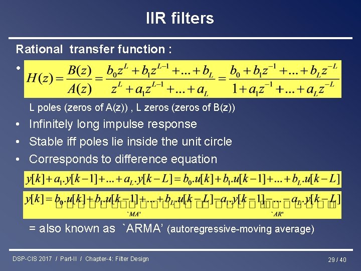
IIR filters Rational transfer function : • L poles (zeros of A(z)) , L zeros (zeros of B(z)) • Infinitely long impulse response • Stable iff poles lie inside the unit circle • Corresponds to difference equation = also known as `ARMA’ (autoregressive-moving average) DSP-CIS 2017 / Part-II / Chapter-4: Filter Design 29 / 40

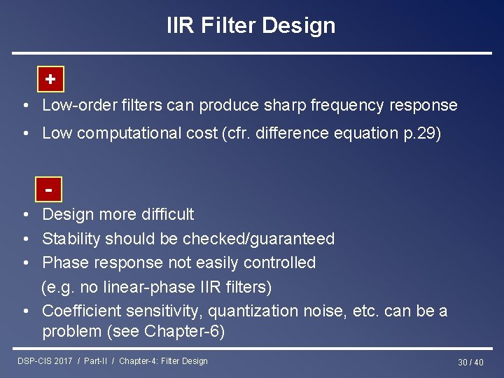
IIR Filter Design + • Low-order filters can produce sharp frequency response • Low computational cost (cfr. difference equation p. 29) • Design more difficult • Stability should be checked/guaranteed • Phase response not easily controlled (e. g. no linear-phase IIR filters) • Coefficient sensitivity, quantization noise, etc. can be a problem (see Chapter-6) DSP-CIS 2017 / Part-II / Chapter-4: Filter Design 30 / 40

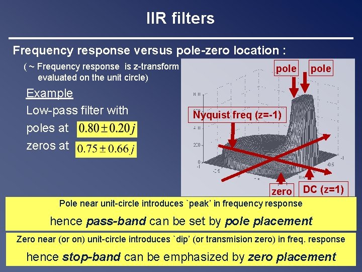
IIR filters Frequency response versus pole-zero location : ( ~ Frequency response is z-transform evaluated on the unit circle) Example Low-pass filter with poles at zeros at pole Nyquist freq (z=-1) zero DC (z=1) Pole near unit-circle introduces `peak’ in frequency response hence pass-band can be set by pole placement Zero near (or on) unit-circle introduces `dip’ (or transmision zero) in freq. response hence stop-band can be emphasized by zero placement 31 / 40 DSP-CIS 2017 / Part-II / Chapter-4: Filter Design

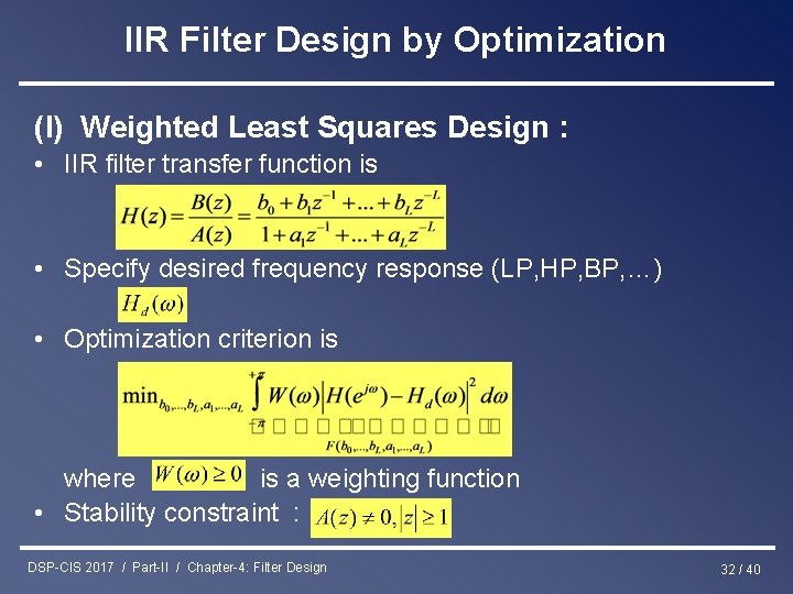
IIR Filter Design by Optimization (I) Weighted Least Squares Design : • IIR filter transfer function is • Specify desired frequency response (LP, HP, BP, …) • Optimization criterion is where is a weighting function • Stability constraint : DSP-CIS 2017 / Part-II / Chapter-4: Filter Design 32 / 40

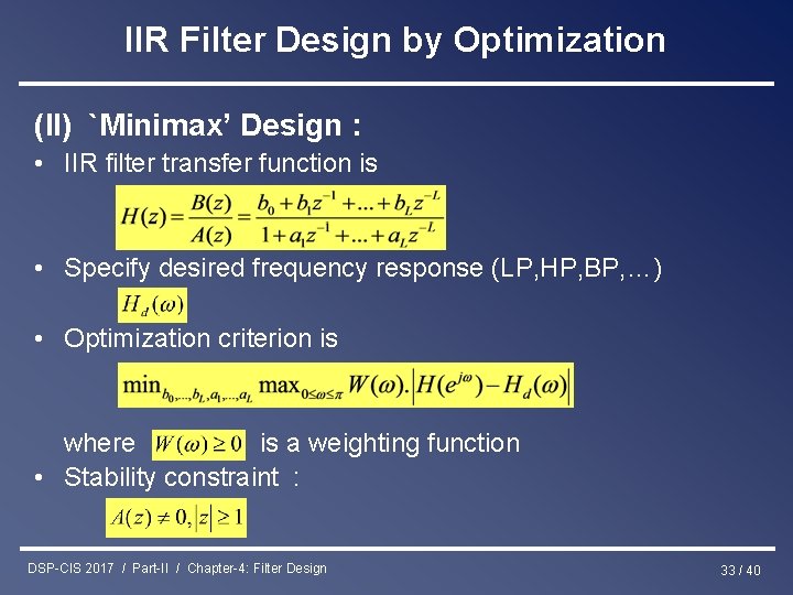
IIR Filter Design by Optimization (II) `Minimax’ Design : • IIR filter transfer function is • Specify desired frequency response (LP, HP, BP, …) • Optimization criterion is where is a weighting function • Stability constraint : DSP-CIS 2017 / Part-II / Chapter-4: Filter Design 33 / 40

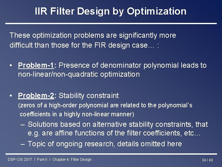
IIR Filter Design by Optimization These optimization problems are significantly more difficult than those for the FIR design case… : • Problem-1: Presence of denominator polynomial leads to non-linear/non-quadratic optimization • Problem-2: Stability constraint (zeros of a high-order polynomial are related to the polynomial’s coefficients in a highly non-linear manner) – Solutions based on alternative stability constraints, that e. g. are affine functions of the filter coefficients, etc… – Topic of ongoing research, details omitted here DSP-CIS 2017 / Part-II / Chapter-4: Filter Design 34 / 40

IIR Filter Design by Optimization • Conclusion: (I) Weighted least squares design (II) Minimax design provide general `framework’, procedures to translate filter design problems into ``standard’’ optimization problems • In practice (and in textbooks): Emphasis on specific (ad-hoc) procedures : - IIR filter design based analog filter design (Butterworth, Chebyshev, elliptic, …) and analog->digital conversion - IIR filter design by modeling = direct z-domain design (Pade approximation, Prony, etc. , not addressed here) DSP-CIS 2017 / Part-II / Chapter-4: Filter Design 35 / 40

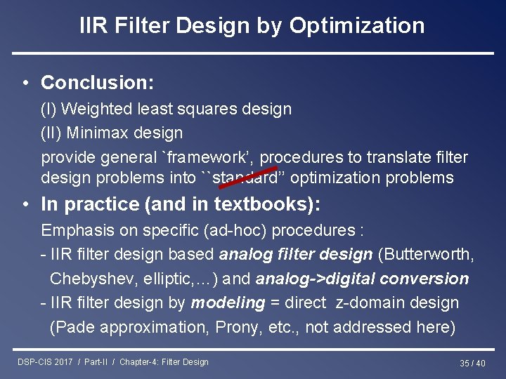
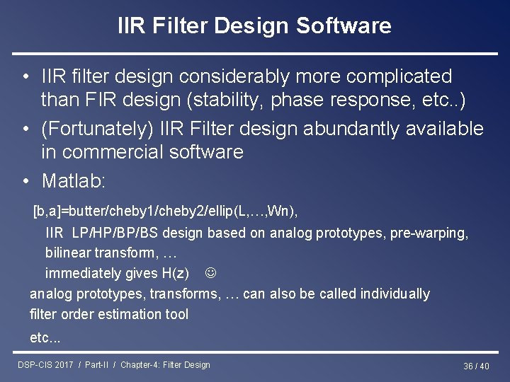
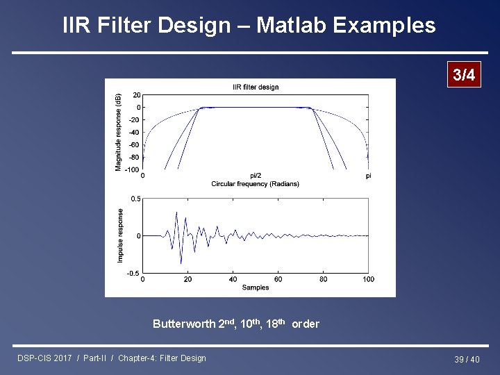
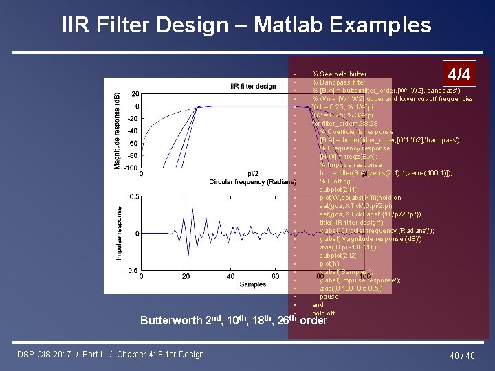
IIR Filter Design Software • IIR filter design considerably more complicated than FIR design (stability, phase response, etc. . ) • (Fortunately) IIR Filter design abundantly available in commercial software • Matlab: [b, a]=butter/cheby 1/cheby 2/ellip(L, …, Wn), IIR LP/HP/BP/BS design based on analog prototypes, pre-warping, bilinear transform, … immediately gives H(z) analog prototypes, transforms, … can also be called individually filter order estimation tool etc. . . DSP-CIS 2017 / Part-II / Chapter-4: Filter Design 36 / 40

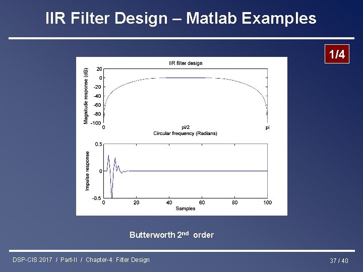
IIR Filter Design – Matlab Examples 1/4 Butterworth 2 nd order DSP-CIS 2017 / Part-II / Chapter-4: Filter Design 37 / 40

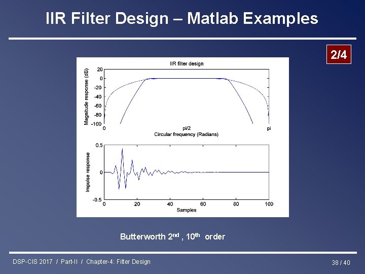
IIR Filter Design – Matlab Examples 2/4 Butterworth 2 nd , 10 th order DSP-CIS 2017 / Part-II / Chapter-4: Filter Design 38 / 40

IIR Filter Design – Matlab Examples 3/4 Butterworth 2 nd, 10 th, 18 th order DSP-CIS 2017 / Part-II / Chapter-4: Filter Design 39 / 40

IIR Filter Design – Matlab Examples Butterworth DSP-CIS 2017 / Part-II / Chapter-4: Filter Design • • • • • • • • 2 nd, 10 th, 18 th, 26 th 4/4 % See help butter % Bandpass filter % [B, A] = butter(filter_order, [W 1 W 2], 'bandpass'); % Wn = [W 1 W 2] upper and lower cut-off frequencies W 1 = 0. 25; % 1/4*pi W 2 = 0. 75; % 3/4*pi for filter_order=2: 8: 28 % Coefficients response [B, A] = butter(filter_order, [W 1 W 2], 'bandpass'); % Frequency response [H W] = freqz(B, A); % Impulse response h = filter(B, A, [zeros(2, 1); 1; zeros(100, 1)]); % Plotting subplot(211) plot(W, db(abs(H))); hold on set(gca, 'XTick', 0: pi/2: pi) set(gca, 'XTick. Label', {'0', 'pi/2', 'pi'}) title('IIR filter design'); xlabel('Circular frequency (Radians)'); ylabel('Magnitude response (d. B)'); axis([0 pi -100 20]) subplot(212) plot(h) xlabel('Samples'); ylabel('Impulse response'); axis([0 100 -0. 5]) pause end hold off order 40 / 40