Dr T presents Evolutionary Computing Computer Science 348

Dr. T presents… Evolutionary Computing Computer Science 348

Introduction • The field of Evolutionary Computing studies theory and application of Evolutionary Algorithms. • Evolutionary Algorithms can be described as a class of stochastic, population-based local search algorithms inspired by neo. Darwinian Evolution Theory.

Computational Basis o Trial-and-error (aka Generate-and-test) o Graduated solution quality o Stochastic local search of adaptive solution landscape o Local vs. global optima o Unimodal vs. multimodal problems

Biological Metaphors o Darwinian Evolution n n Macroscopic view of evolution Natural selection Survival of the fittest Random variation

Biological Metaphors o (Mendelian) Genetics n Genotype (functional unit of inheritance) n Genotypes vs. phenotypes n Pleitropy: one gene affects multiple phenotypic traits n Polygeny: one phenotypic trait is affected by multiple genes n Chromosomes (haploid vs. diploid) n Loci and alleles

Computational Problem Classes o Optimization problems o Modeling (aka system identification) problems o Simulation problems

EA Pros o More general purpose than traditional optimization algorithms; i. e. , less problem specific knowledge required o Ability to solve “difficult” problems o Solution availability o Robustness o Inherent parallelism

EA Cons o Fitness function and genetic operators often not obvious o Premature convergence o Computationally intensive o Difficult parameter optimization

EA components o Search spaces: representation & size o Evaluation of trial solutions: fitness function o Exploration versus exploitation o Selective pressure rate o Premature convergence

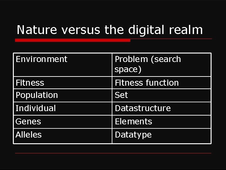
Nature versus the digital realm Environment Problem (search space) Fitness Population Fitness function Set Individual Datastructure Genes Elements Alleles Datatype

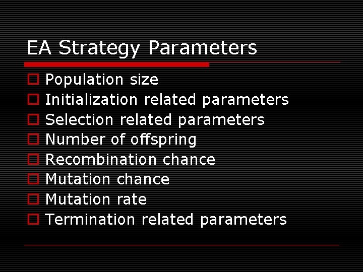
EA Strategy Parameters o o o o Population size Initialization related parameters Selection related parameters Number of offspring Recombination chance Mutation rate Termination related parameters

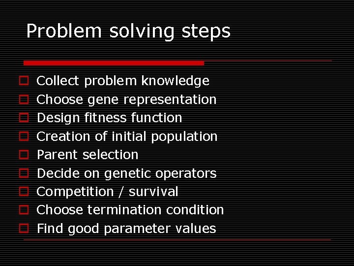
Problem solving steps o o o o o Collect problem knowledge Choose gene representation Design fitness function Creation of initial population Parent selection Decide on genetic operators Competition / survival Choose termination condition Find good parameter values

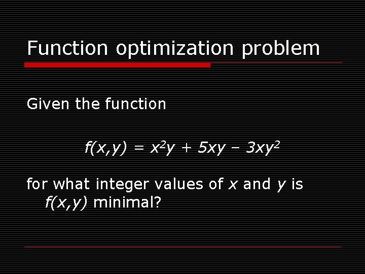
Function optimization problem Given the function f(x, y) = x 2 y + 5 xy – 3 xy 2 for what integer values of x and y is f(x, y) minimal?

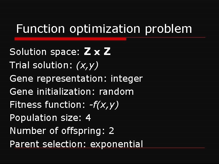
Function optimization problem Solution space: Z x Z Trial solution: (x, y) Gene representation: integer Gene initialization: random Fitness function: -f(x, y) Population size: 4 Number of offspring: 2 Parent selection: exponential

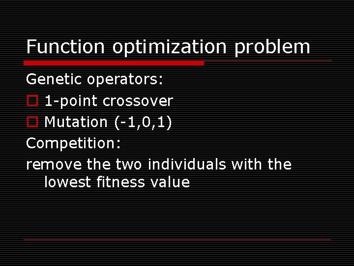
Function optimization problem Genetic operators: o 1 -point crossover o Mutation (-1, 0, 1) Competition: remove the two individuals with the lowest fitness value

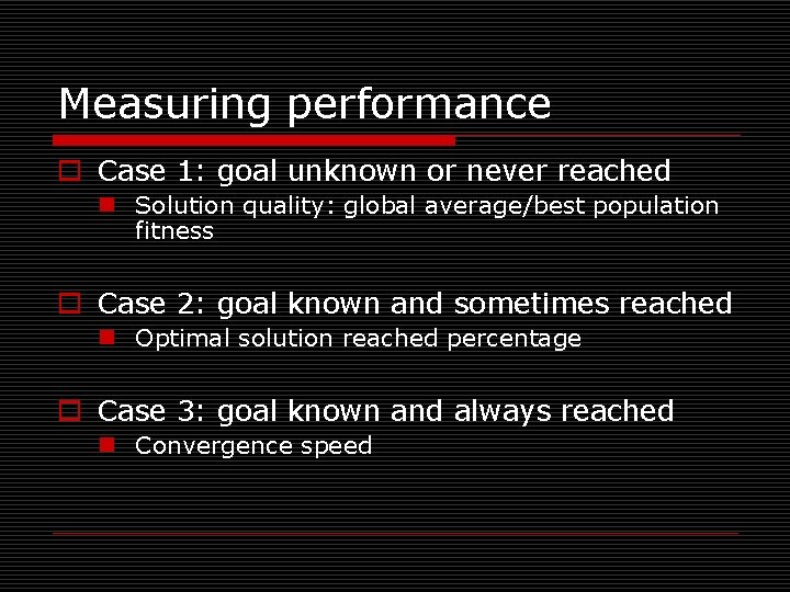
Measuring performance o Case 1: goal unknown or never reached n Solution quality: global average/best population fitness o Case 2: goal known and sometimes reached n Optimal solution reached percentage o Case 3: goal known and always reached n Convergence speed

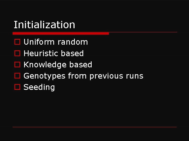
Initialization o o o Uniform random Heuristic based Knowledge based Genotypes from previous runs Seeding

Representation (§ 2. 3. 1) o o o Genotype space Phenotype space Encoding & Decoding Knapsack Problem (§ 2. 4. 2) Surjective, injective, and bijective decoder functions

Simple Genetic Algorithm (SGA) o o o Representation: Bit-strings Recombination: 1 -Point Crossover Mutation: Bit Flip Parent Selection: Fitness Proportional Survival Selection: Generational

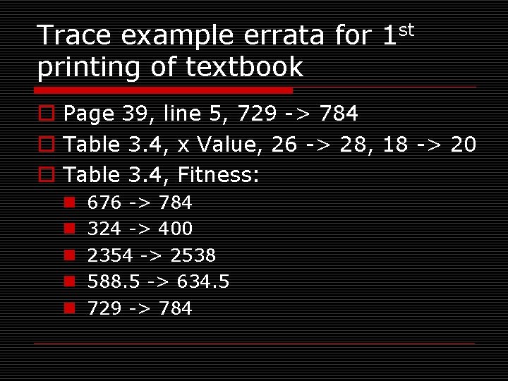
Trace example errata for 1 st printing of textbook o Page 39, line 5, 729 -> 784 o Table 3. 4, x Value, 26 -> 28, 18 -> 20 o Table 3. 4, Fitness: n n n 676 -> 784 324 -> 400 2354 -> 2538 588. 5 -> 634. 5 729 -> 784

Representations o Bit Strings n Scaling Hamming Cliffs n Binary vs. Gray coding (Appendix A) o Integers n Ordinal vs. cardinal attributes n Permutations o Absolute order vs. adjacency o Real-Valued, etc. o Homogeneous vs. heterogeneous

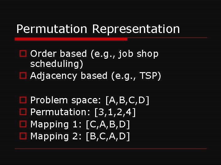
Permutation Representation o Order based (e. g. , job shop scheduling) o Adjacency based (e. g. , TSP) o o Problem space: [A, B, C, D] Permutation: [3, 1, 2, 4] Mapping 1: [C, A, B, D] Mapping 2: [B, C, A, D]

Mutation vs. Recombination o Mutation = Stochastic unary variation operator o Recombination = Stochastic multi-ary variation operator

Mutation o Bit-String Representation: n Bit-Flip n E[#flips] = L * pm o Integer Representation: n Random Reset (cardinal attributes) n Creep Mutation (ordinal attributes)

Mutation cont. o Floating-Point n Uniform n Nonuniform from fixed distribution o Gaussian, Cauche, Levy, etc.

Permutation Mutation o o Swap Mutation Insert Mutation Scramble Mutation Inversion Mutation (good for adjacency based problems)

Recombination o o o o Recombination rate: asexual vs. sexual N-Point Crossover (positional bias) Uniform Crossover (distributional bias) Discrete recombination (no new alleles) (Uniform) arithmetic recombination Simple recombination Single arithmetic recombination Whole arithmetic recombination

Permutation Recombination Adjacency based problems o Partially Mapped Crossover (PMX) o Edge Crossover Order based problems o Order Crossover o Cycle Crossover

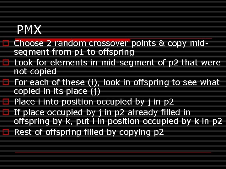
PMX o Choose 2 random crossover points & copy midsegment from p 1 to offspring o Look for elements in mid-segment of p 2 that were not copied o For each of these (i), look in offspring to see what copied in its place (j) o Place i into position occupied by j in p 2 o If place occupied by j in p 2 already filled in offspring by k, put i in position occupied by k in p 2 o Rest of offspring filled by copying p 2

Order Crossover o Choose 2 random crossover points & copy mid-segment from p 1 to offspring o Starting from 2 nd crossover point in p 2, copy unused numbers into offspring in the order they appear in p 2, wrapping around at end of list

Population Models o Two historical models n Generational Model n Steady State Model o Generational Gap o General model n Population size n Mating pool size n Offspring pool size

Parent selection o Random o Fitness Based n Proportional Selection (FPS) n Rank-Based Selection o Genotypic/phenotypic Based

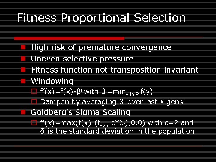
Fitness Proportional Selection n n High risk of premature convergence Uneven selective pressure Fitness function not transposition invariant Windowing o f’(x)=f(x)-βt with βt=miny in Ptf(y) o Dampen by averaging βt over last k gens n Goldberg’s Sigma Scaling o f’(x)=max(f(x)-(favg-c*δf), 0. 0) with c=2 and δf is the standard deviation in the population

Rank-Based Selection n Mapping function (ala SA cooling schedule) n Exponential Ranking n Linear ranking

Sampling methods o Roulette Wheel o Stochastic Universal Sampling (SUS)

Rank based sampling methods o Tournament Selection n Tournament Size

Survivor selection o Age-based o Fitness-based n Truncation o Elitism

Termination o o o CPU time / wall time Number of fitness evaluations Lack of fitness improvement Lack of genetic diversity Solution quality / solution found Combination of the above

Behavioral observables o Selective pressure o Population diversity n n Fitness values Phenotypes Genotypes Alleles

Multi-Objective EAs (MOEAs) o Extension of regular EA which maps multiple objective values to single fitness value o Objectives typically conflict o In a standard EA, an individual A is said to be better than an individual B if A has a higher fitness value than B o In a MOEA, an individual A is said to be better than an individual B if A dominates B

Domination in MOEAs o An individual A is said to dominate individual B iff: n A is no worse than B in all objectives n A is strictly better than B in at least one objective

Pareto Optimality (Vilfredo Pareto) o Given a set of alternative allocations of, say, goods or income for a set of individuals, a movement from one allocation to another that can make at least one individual better off without making any other individual worse off is called a Pareto Improvement. An allocation is Pareto Optimal when no further Pareto Improvements can be made. This is often called a Strong Pareto Optimum (SPO).

Pareto Optimality in MOEAs o Among a set of solutions P, the nondominated subset of solutions P’ are those that are not dominated by any member of the set P o The non-dominated subset of the entire feasible search space S is the globally Pareto-optimal set

Goals of MOEAs o Identify the Global Pareto-Optimal set of solutions (aka the Pareto Optimal Front) o Find a sufficient coverage of that set o Find an even distribution of solutions

MOEA metrics o Convergence: How close is a generated solution set to the true Pareto-optimal front o Diversity: Are the generated solutions evenly distributed, or are they in clusters

Deterioration in MOEAs o Competition can result in the loss of a non-dominated solution which dominated a previously generated solution o This loss in its turn can result in the previously generated solution being regenerated and surviving

NSGA-II o Initialization – before primary loop Create initial population P 0 Sort P 0 on the basis of non-domination Best level is level 1 Fitness is set to level number; lower number, higher fitness n Binary Tournament Selection n Mutation and Recombination create Q 0 n n

NSGA-II (cont. ) o Primary Loop n Rt = P t + Q t n Sort Rt on the basis of non-domination n Create Pt + 1 by adding the best individuals from Rt n Create Qt + 1 by performing Binary Tournament Selection, Recombination, and Mutation on Pt + 1

NSGA-II (cont. ) o Crowding distance metric: average side length of cuboid defined by nearest neighbors in same front o Parent tournament selection employs crowding distance as a tie breaker

Epsilon-MOEA o Steady State o Elitist o No deterioration

Epsilon-MOEA (cont. ) o Create an initial population P(0) o Epsilon non-dominated solutions from P(0) are put into an archive population E(0) o Choose one individual from E, and one from P o These individuals mate and produce an offspring, c o A special array B is created for c, which consists of abbreviated versions of the objective values from c

Epsilon-MOEA (cont. ) o An attempt to insert c into the archive population E o The domination check is conducted using the B array instead of the actual objective values o If c dominates a member of the archive, that member will be replaced with c o The individual c can also be inserted into P in a similar manner using a standard domination check

SNDL-MOEA o Desired Features n n n n Deterioration Prevention Stored non-domination levels (NSGA-II) Number and size of levels user configurable Selection methods utilizing levels in different ways Problem specific representation Problem specific “compartments” (E-MOEA) Problem specific mutation and crossover

Report writing tips o Use easily readable fonts, including in tables & graphs (11 pnt fonts are typically best, 10 pnt is the absolute smallest) o Number all figures and tables and refer to each and every one in the main text body (hint: use autonumbering) o Capitalize named articles (e. g. , ``see Table 5'', not ``see table 5'') o Keep important figures and tables as close to the referring text as possible, while placing less important ones in an appendix o Always provide standard deviations (typically in between parentheses) when listing averages

Report writing tips o Use descriptive titles, captions on tables and figures so that they are self-explanatory o Always include axis labels in graphs o Write in a formal style (never use first person, instead say, for instance, ``the author'') o Format tabular material in proper tables with grid lines o Avoid making explicit physical layout references like “in the below table” or “in the figure on the next page”; instead use logical layout references like “in Table” or “in the previous paragraph” o Provide all the required information, but avoid extraneous data (information is good, data is bad)

Evolutionary Programming (EP) o Traditional application domain: machine learning by FSMs o Contemporary application domain: (numerical) optimization o arbitrary representation and mutation operators, no recombination o contemporary EP = traditional EP + ES n self-adaptation of parameters

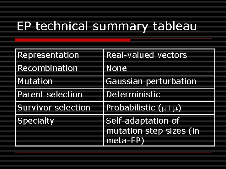
EP technical summary tableau Representation Real-valued vectors Recombination None Mutation Gaussian perturbation Parent selection Deterministic Survivor selection Probabilistic ( + ) Specialty Self-adaptation of mutation step sizes (in meta-EP)

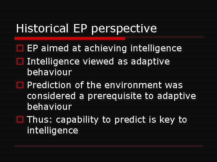
Historical EP perspective o EP aimed at achieving intelligence o Intelligence viewed as adaptive behaviour o Prediction of the environment was considered a prerequisite to adaptive behaviour o Thus: capability to predict is key to intelligence

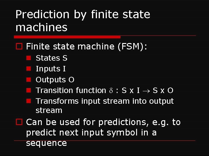
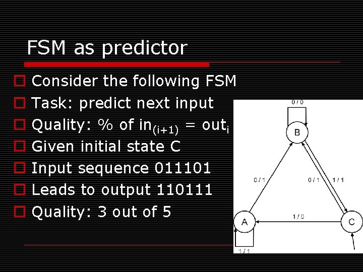
Prediction by finite state machines o Finite state machine (FSM): n n n States S Inputs I Outputs O Transition function : S x I S x O Transforms input stream into output stream o Can be used for predictions, e. g. to predict next input symbol in a sequence

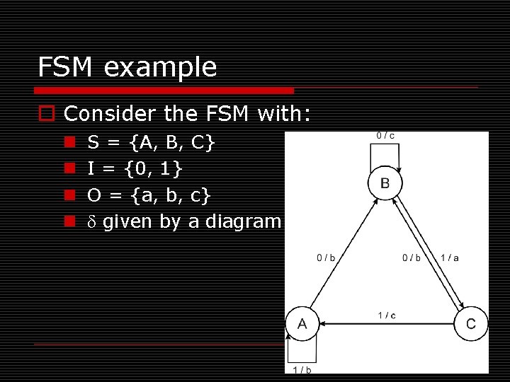
FSM example o Consider the FSM with: n n S = {A, B, C} I = {0, 1} O = {a, b, c} given by a diagram

FSM as predictor o o o o Consider the following FSM Task: predict next input Quality: % of in(i+1) = outi Given initial state C Input sequence 011101 Leads to output 110111 Quality: 3 out of 5

Introductory example: evolving FSMs to predict primes o o o P(n) = 1 if n is prime, 0 otherwise I = N = {1, 2, 3, …, n, …} O = {0, 1} Correct prediction: outi= P(in(i+1)) Fitness function: n 1 point for correct prediction of next input n 0 point for incorrect prediction n Penalty for “too many” states

Introductory example: evolving FSMs to predict primes o Parent selection: each FSM is mutated once o Mutation operators (one selected randomly): n n n Change an output symbol Change a state transition (i. e. redirect edge) Add a state Delete a state Change the initial state o Survivor selection: ( + ) o Results: overfitting, after 202 inputs best FSM had one state and both outputs were 0, i. e. , it always predicted “not prime”

Modern EP o No predefined representation in general o Thus: no predefined mutation (must match representation) o Often applies self-adaptation of mutation parameters o In the sequel we present one EP variant, not the canonical EP

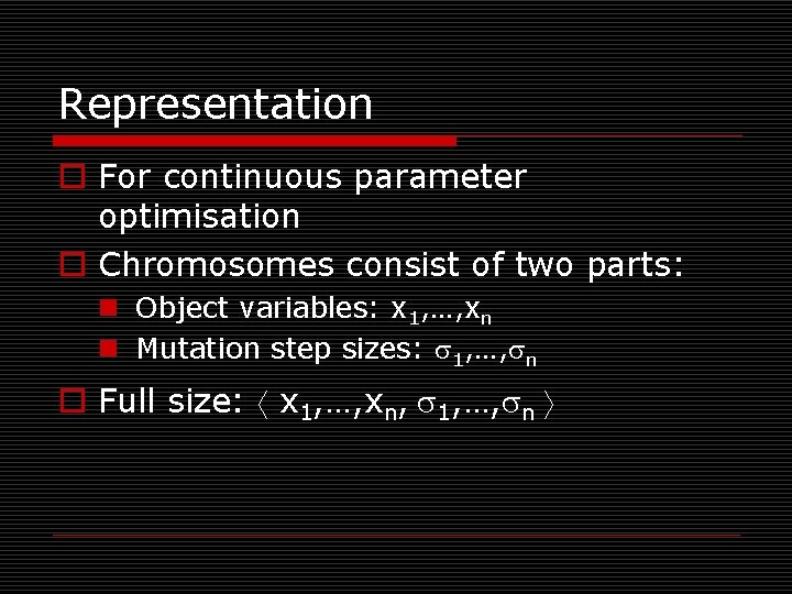
Representation o For continuous parameter optimisation o Chromosomes consist of two parts: n Object variables: x 1, …, xn n Mutation step sizes: 1, …, n o Full size: x 1, …, xn, 1, …, n

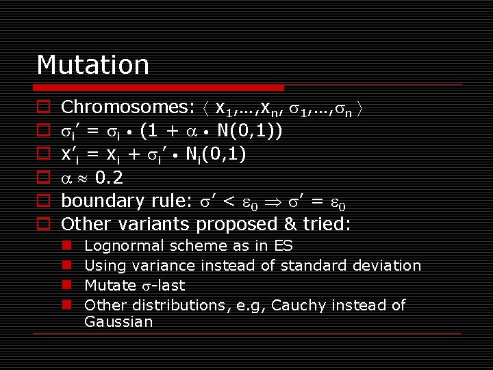
Mutation o o o Chromosomes: x 1, …, xn, 1, …, n i’ = i • (1 + • N(0, 1)) x’i = xi + i’ • Ni(0, 1) 0. 2 boundary rule: ’ < 0 ’ = 0 Other variants proposed & tried: n n Lognormal scheme as in ES Using variance instead of standard deviation Mutate -last Other distributions, e. g, Cauchy instead of Gaussian

Recombination o None o Rationale: one point in the search space stands for a species, not for an individual and there can be no crossover between species o Much historical debate “mutation vs. crossover” o Pragmatic approach seems to prevail today

Parent selection o Each individual creates one child by mutation o Thus: n Deterministic n Not biased by fitness

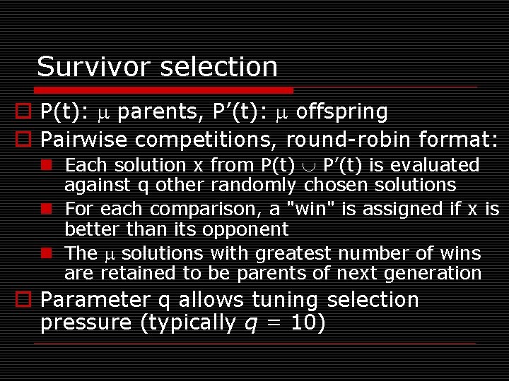
Survivor selection o P(t): parents, P’(t): offspring o Pairwise competitions, round-robin format: n Each solution x from P(t) P’(t) is evaluated against q other randomly chosen solutions n For each comparison, a "win" is assigned if x is better than its opponent n The solutions with greatest number of wins are retained to be parents of next generation o Parameter q allows tuning selection pressure (typically q = 10)

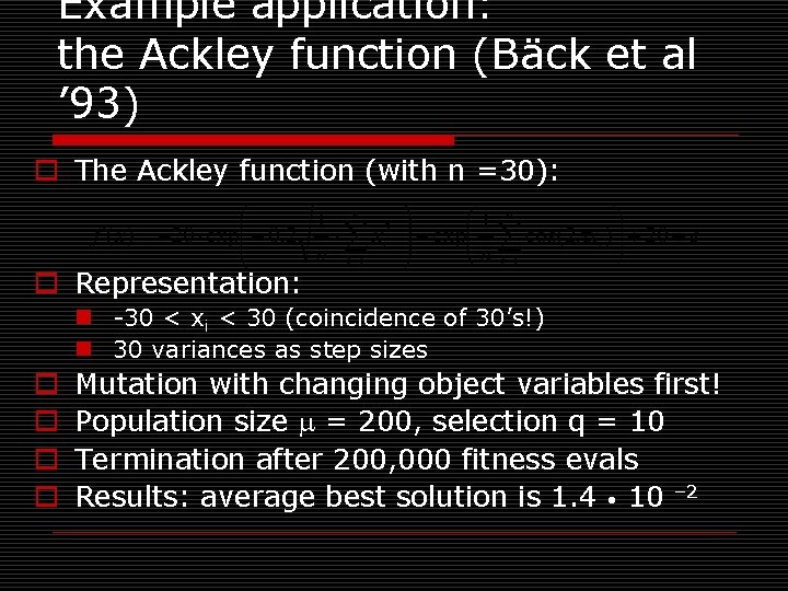
Example application: the Ackley function (Bäck et al ’ 93) o The Ackley function (with n =30): o Representation: n -30 < xi < 30 (coincidence of 30’s!) n 30 variances as step sizes o o Mutation with changing object variables first! Population size = 200, selection q = 10 Termination after 200, 000 fitness evals Results: average best solution is 1. 4 • 10 – 2

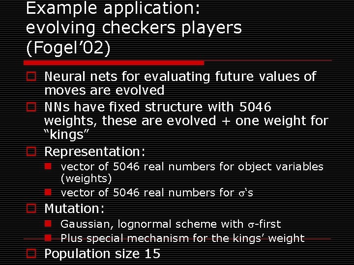
Example application: evolving checkers players (Fogel’ 02) o Neural nets for evaluating future values of moves are evolved o NNs have fixed structure with 5046 weights, these are evolved + one weight for “kings” o Representation: n vector of 5046 real numbers for object variables (weights) n vector of 5046 real numbers for ‘s o Mutation: n Gaussian, lognormal scheme with -first n Plus special mechanism for the kings’ weight o Population size 15

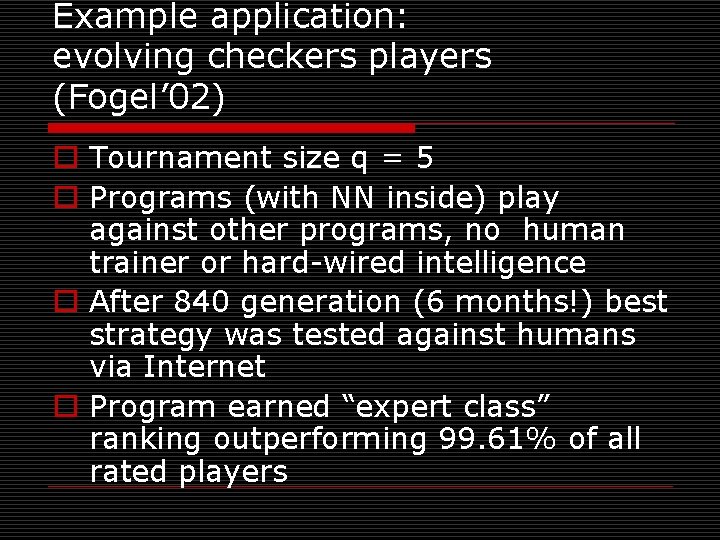
Example application: evolving checkers players (Fogel’ 02) o Tournament size q = 5 o Programs (with NN inside) play against other programs, no human trainer or hard-wired intelligence o After 840 generation (6 months!) best strategy was tested against humans via Internet o Program earned “expert class” ranking outperforming 99. 61% of all rated players

Deriving Gas-Phase Exposure History through Computationally Evolved Inverse Diffusion Analysis o Joshua M. Eads o Former undergraduate student in Computer Science o Daniel Tauritz o Associate Professor of Computer Science o Glenn Morrison o Associate Professor of Environmental Engineering o Ekaterina Smorodkina o Former Ph. D. Student in Computer Science

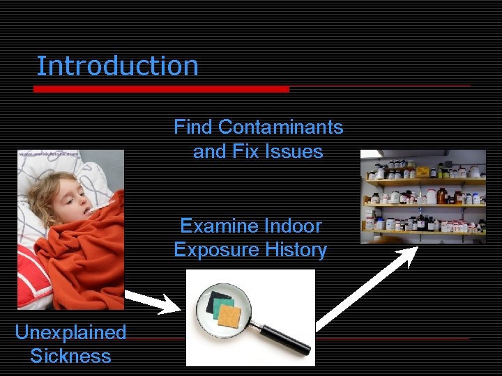
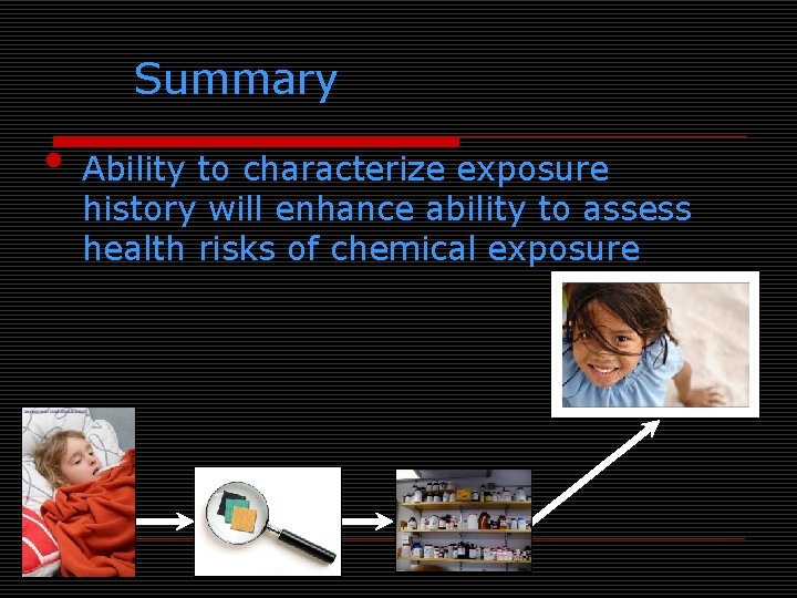
Introduction Find Contaminants and Fix Issues Examine Indoor Exposure History Unexplained Sickness

Background • • Indoor air pollution top five environmental health risks $160 billion could be saved every year by improving indoor air quality Current exposure history is inadequate A reliable method is needed to determine past contamination levels and times

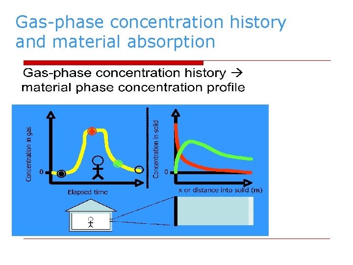
Problem Statement • A forward diffusion differential equation predicts concentration in materials after exposure • An inverse diffusion equation finds the timing and intensity of previous gas contamination • Knowledge of early exposures would greatly strengthen epidemiological conclusions

Gas-phase concentration history and material absorption

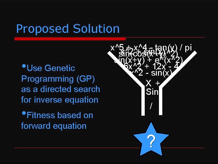
Proposed Solution • Use Genetic Programming (GP) as a directed search for inverse equation • Fitness based on x^5 x^2 + x^4 - tan(y) / pi + sin(x) sin(cos(x+y)^2) sin(x+y) + e^(x^2) 5 x^2 + 12 x - 4 x^2 - sin(x) X + Sin / forward equation ?

Related Research • • • It has been proven that the inverse equation exists Symbolic regression with GP has successfully found both differential equations and inverse functions Similar inverse problems in thermodynamics and geothermal research have been solved

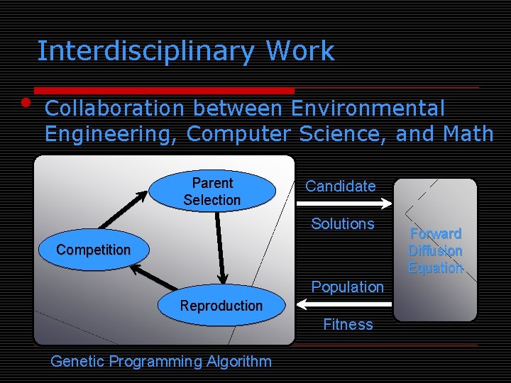
Interdisciplinary Work • Collaboration between Environmental Engineering, Computer Science, and Math Parent Selection Candidate Solutions Competition Population Reproduction Fitness Genetic Programming Algorithm Forward Diffusion Equation

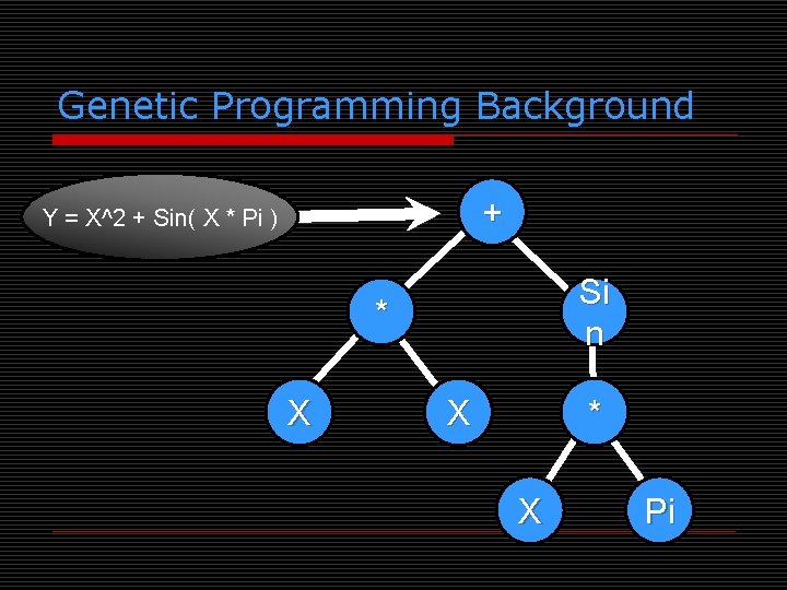
Genetic Programming Background + Y = X^2 + Sin( X * Pi ) Si n * X X * X Pi

Summary • Ability to characterize exposure history will enhance ability to assess health risks of chemical exposure

Genetic Programming (GP) o Characteristic property: variable-size hierarchical representation vs. fixedsize linear in traditional EAs o Application domain: model optimization vs. input values in traditional EAs o Unifying Paradigm: Program Induction

Program induction examples o o o o o Optimal control Planning Symbolic regression Automatic programming Discovering game playing strategies Forecasting Inverse problem solving Decision Tree induction Evolution of emergent behavior Evolution of cellular automata

GP specification o o o o S-expressions Function set Terminal set Arity Correct expressions Closure property Strongly typed GP

GP notes o Mutation or recombination (not both) o Bloat (survival of the fattest) o Parsimony pressure

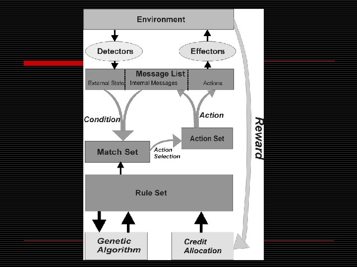
Learning Classifier Systems (LCS) o Note: LCS is technically not a type of EA, but can utilize an EA o Condition-Action Rule Based Systems n rule format: <condition: action> o Reinforcement Learning o LCS rule format: n <condition: action> → predicted payoff n don’t care symbols

LCS specifics o Multi-step credit allocation – Bucket Brigade algorithm o Rule Discovery Cycle – EA o Pitt approach: each individual represents a complete rule set o Michigan approach: each individual represents a single rule, a population represents the complete rule set

Parameter Tuning methods o Start with stock parameter values o Manually adjust based on user intuition o Monte Carlo sampling of parameter values on a few (short) runs o Tuning algorithm (e. g. , REVAC which employs an information theoretic measure on how sensitive performance is to the choice of a parameter’s value) o Meta-tuning algorithm (e. g. , meta-EA)

Parameter Tuning Challenges o Exhaustive search for optimal values of parameters, even assuming independency, is infeasible o Parameter dependencies o Extremely time consuming o Optimal values are very problem specific

Static vs. dynamic parameters o The optimal value of a parameter can change during evolution o Static parameters remain constant during evolution, dynamic parameters can change o Dynamic parameters require parameter control

Tuning vs Control confusion o Parameter Tuning: A priori optimization of fixed strategy parameters o Parameter Control: On-the-fly optimization of dynamic strategy parameters

Parameter Control o While dynamic parameters can benefit from tuning, performance tends to be much less sensitive to initial values for dynamic parameters than static o Controls dynamic parameters o Three main parameter control classes: n Blind n Adaptive n Self-Adaptive

Parameter Control methods o Blind (termed “deterministic” in textbook) n Example: replace pi with pi(t) o akin to cooling schedule in Simulated Annealing o Adaptive n Example: Rechenberg’s 1/5 success rule o Self-adaptive n Example: Mutation-step size control in ES

Evaluation Function Control o Example 1: Parsimony Pressure in GP o Example 2: Penalty Functions in Constraint Satisfaction Problems (aka Constrained Optimization Problems)

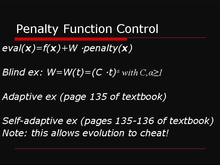
Penalty Function Control eval(x)=f(x)+W ·penalty(x) Blind ex: W=W(t)=(C ·t)α with C, α≥ 1 Adaptive ex (page 135 of textbook) Self-adaptive ex (pages 135 -136 of textbook) Note: this allows evolution to cheat!

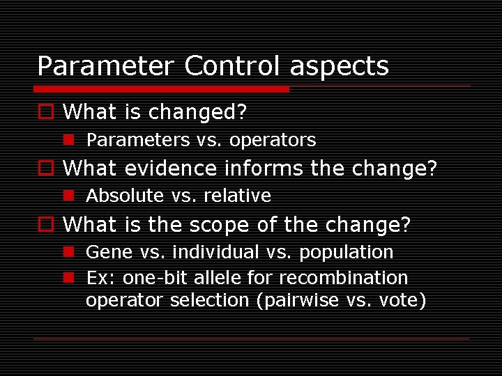
Parameter Control aspects o What is changed? n Parameters vs. operators o What evidence informs the change? n Absolute vs. relative o What is the scope of the change? n Gene vs. individual vs. population n Ex: one-bit allele for recombination operator selection (pairwise vs. vote)

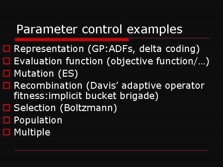
Parameter control examples Representation (GP: ADFs, delta coding) Evaluation function (objective function/…) Mutation (ES) Recombination (Davis’ adaptive operator fitness: implicit bucket brigade) o Selection (Boltzmann) o Population o Multiple o o

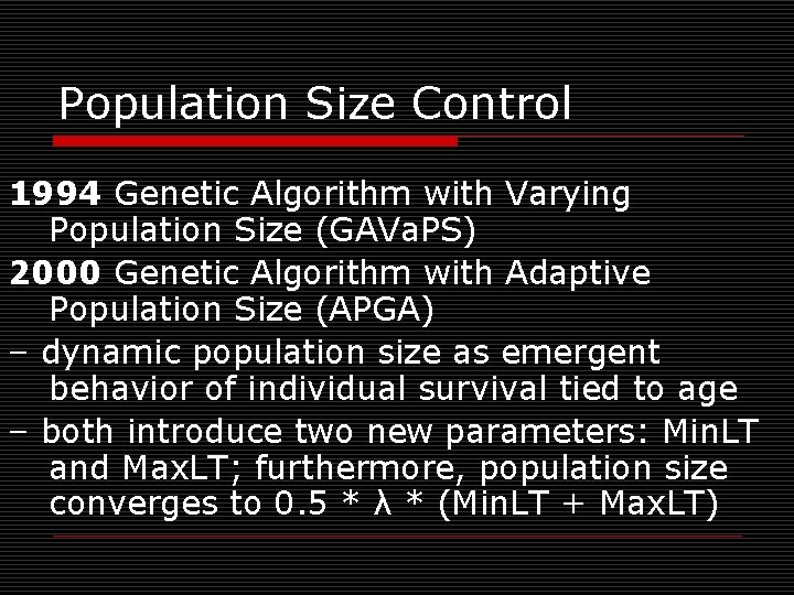
Population Size Control 1994 Genetic Algorithm with Varying Population Size (GAVa. PS) 2000 Genetic Algorithm with Adaptive Population Size (APGA) – dynamic population size as emergent behavior of individual survival tied to age – both introduce two new parameters: Min. LT and Max. LT; furthermore, population size converges to 0. 5 * λ * (Min. LT + Max. LT)

Population Size Control 1995 (1, λ)-ES with dynamic offspring size employing adaptive control – adjusts λ based on the second best individual created – goal is to maximize local serial progressrate, i. e. , expected fitness gain per fitness evaluation – maximizes convergence rate, which often leads to premature convergence on complex fitness landscapes

Population Size Control 1999 Parameter-less GA – runs multiple fixed size populations in parallel – the sizes are powers of 2, starting with 4 and doubling the size of the largest population to produce the next largest population – smaller populations are preferred by allotting them more generations – a population is deleted if a) its average fitness is exceeded by the average fitness of a larger population, or b) the population has converged

Population Size Control 2003 self-adaptive selection of reproduction operators – each individual contains a vector of probabilities of using each reproduction operator defined for the problem – probability vectors updated every generation – in the case of a multi-ary reproduction operator, another individual is selected which prefers the same reproduction operator

Population Size Control 2004 Population Resizing on Fitness Improvement GA (PRo. FIGA) – dynamically balances exploration versus exploitation by tying population size to magnitude of fitness increases with a special mechanism to escape local optima – introduces several new parameters

Population Size Control 2005 (1+λ)-ES with dynamic offspring size employing adaptive control – adjusts λ based on the number of offspring fitter than their parent: if none fitter, than double λ; otherwise divide λ by number that are fitter – idea is to quickly increase λ when it appears to be too small, otherwise to decrease it based on the current success rate – has problems with complex fitness landscapes that require a large λ to ensure

Population Size Control 2006 self-adaptation of population size and selective pressure – employs “voting system” by encoding individual’s contribution to population size in its genotype – population size is determined by summing up all the individual “votes” – adds new parameters pmin and pmax that determine an individual’s vote value range

Motivation for new type of EA o Selection operators are not commonly used in an adaptive manner o Most selection pressure mechanisms are based on Boltzmann selection o Framework for creating Parameterless EAs o Centralized population size control, parent selection, mate pairing, offspring size control, and survival selection are highly unnatural!

Approach for new type of EA Remove unnatural centralized control by: o Letting individuals select their own mates o Letting couples decide how many offspring to have o Giving each individual its own survival chance

Autonomous EAs (Auto. EAs) o An Auto. EA is an EA where all the operators work at the individual level (as opposed to traditional EAs where parent selection and survival selection work at the population level in a decidedly unnatural centralized manner) o Population & offspring size become dynamic derived variables determined by the emergent behavior of the system

Evolution Strategies (ES) o Birth year: 1963 o Birth place: Technical University of Berlin, Germany o Parents: Ingo Rechenberg & Hans. Paul Schwefel

ES history & parameter control o o o Two-membered ES: (1+1) Original multi-membered ES: (µ+1) Multi-membered ES: (µ+λ), (µ, λ) Parameter tuning vs. parameter control Adaptive parameter control n Rechenberg’s 1/5 success rule o Self-adaptation n Mutation Step control

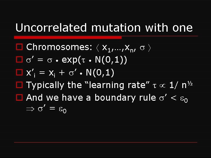
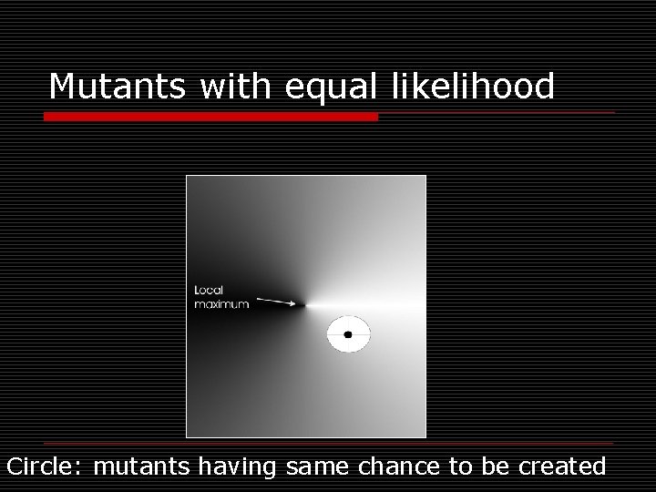
Uncorrelated mutation with one o o o Chromosomes: x 1, …, xn, ’ = • exp( • N(0, 1)) x’i = xi + ’ • N(0, 1) Typically the “learning rate” 1/ n½ And we have a boundary rule ’ < 0 ’ = 0

Mutants with equal likelihood Circle: mutants having same chance to be created

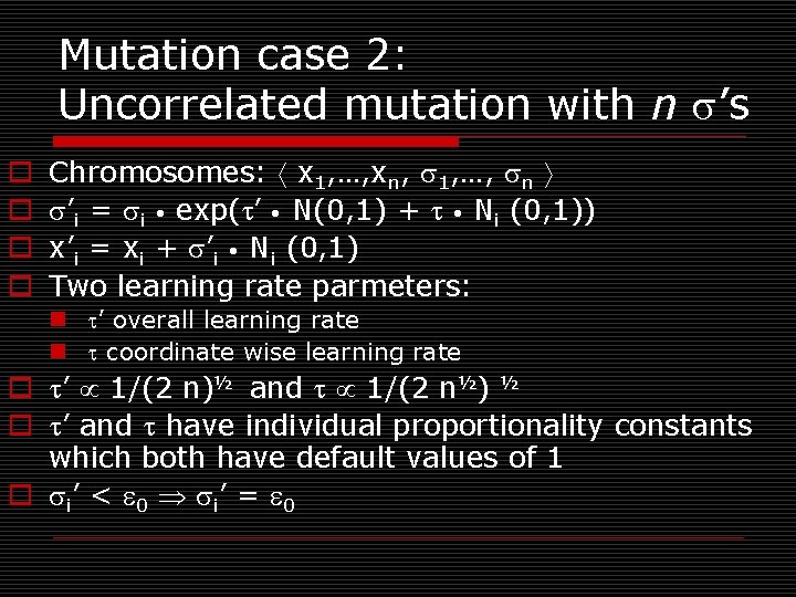
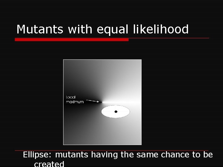
Mutation case 2: Uncorrelated mutation with n ’s o o Chromosomes: x 1, …, xn, 1, …, n ’i = i • exp( ’ • N(0, 1) + • Ni (0, 1)) x’i = xi + ’i • Ni (0, 1) Two learning rate parmeters: n ’ overall learning rate n coordinate wise learning rate o ’ 1/(2 n)½ and 1/(2 n½) ½ o ’ and have individual proportionality constants which both have default values of 1 o i ’ < 0 i ’ = 0

Mutants with equal likelihood Ellipse: mutants having the same chance to be

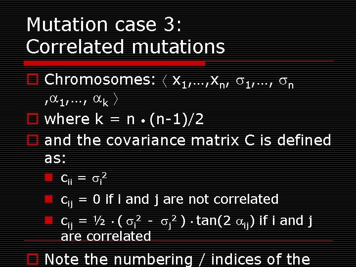
Mutation case 3: Correlated mutations o Chromosomes: x 1, …, xn, 1, …, n , 1, …, k o where k = n • (n-1)/2 o and the covariance matrix C is defined as: n cii = i 2 n cij = 0 if i and j are not correlated n cij = ½ • ( i 2 - j 2 ) • tan(2 ij) if i and j are correlated o Note the numbering / indices of the

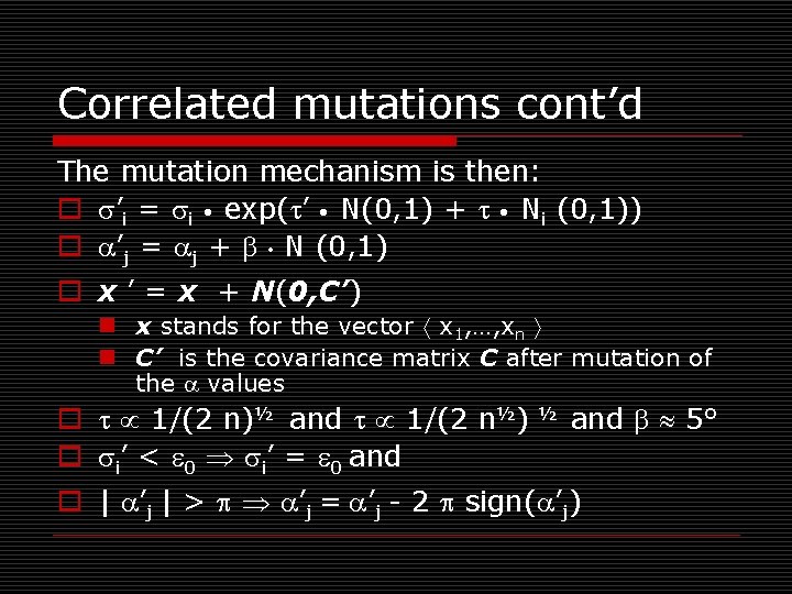
Correlated mutations cont’d The mutation mechanism is then: o ’i = i • exp( ’ • N(0, 1) + • Ni (0, 1)) o ’j = j + • N (0, 1) o x ’ = x + N(0, C’) n x stands for the vector x 1, …, xn n C’ is the covariance matrix C after mutation of the values o 1/(2 n)½ and 1/(2 n½) o i’ < 0 i’ = 0 and ½ and 5° o | ’j | > ’j = ’j - 2 sign( ’j)

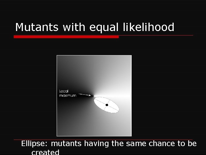
Mutants with equal likelihood Ellipse: mutants having the same chance to be

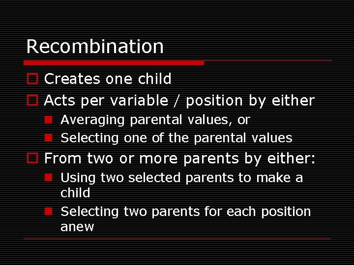
Recombination o Creates one child o Acts per variable / position by either n Averaging parental values, or n Selecting one of the parental values o From two or more parents by either: n Using two selected parents to make a child n Selecting two parents for each position anew

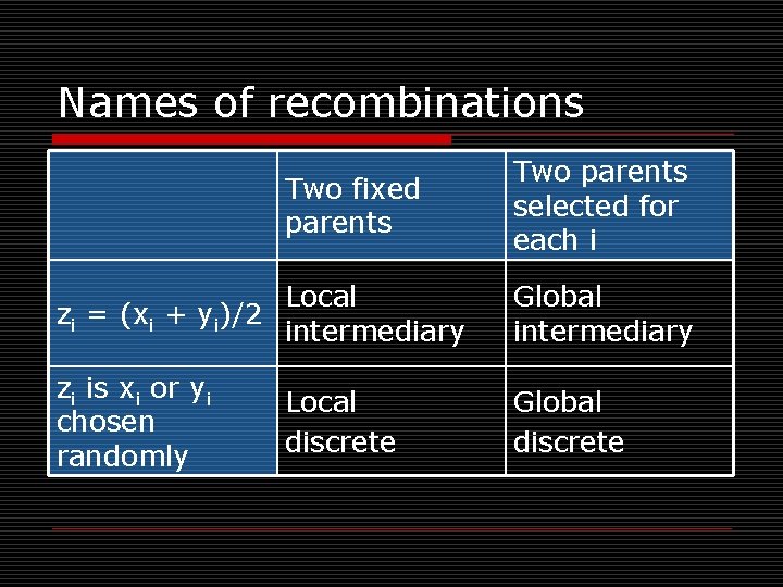
Names of recombinations Two fixed parents Two parents selected for each i Local zi = (xi + yi)/2 intermediary Global intermediary zi is xi or yi chosen randomly Global discrete Local discrete

Multimodal Problems o Multimodal def. : multiple local optima and at least one local optimum is not globally optimal o Adaptive landscapes & neighborhoods o Basins of attraction & Niches o Motivation for identifying a diverse set of high quality solutions: n Allow for human judgment n Sharp peak niches may be overfitted

Restricted Mating o Panmictic vs. restricted mating o Finite pop size + panmictic mating -> genetic drift o Local Adaptation (environmental niche) o Punctuated Equilibria n Evolutionary Stasis n Demes o Speciation (end result of increasingly specialized adaptation to particular environmental niches)

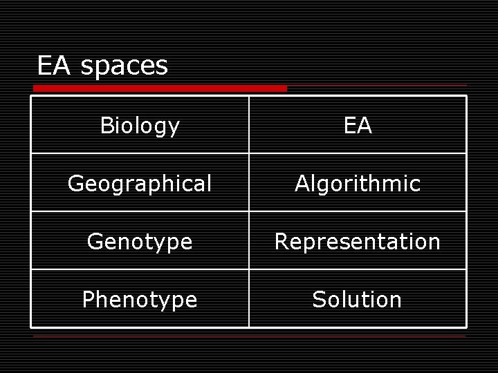
EA spaces Biology EA Geographical Algorithmic Genotype Representation Phenotype Solution

Implicit diverse solution identification (1) o Multiple runs of standard EA n Non-uniform basins of attraction problematic o Island Model (coarse-grain parallel) n n Punctuated Equilibria Epoch, migration Communication characteristics Initialization: number of islands and respective population sizes

Implicit diverse solution identification (2) o Diffusion Model EAs n Single Population, Single Species n Overlapping demes distributed within Algorithmic Space (e. g. , grid) n Equivalent to cellular automata o Automatic Speciation n Genotype/phenotype mating restrictions

Explicit diverse solution identification o Fitness Sharing: individuals share fitness within their niche o Crowding: replace similar parents

Game-Theoretic Problems Adversarial search: multi-agent problem with conflicting utility functions Ultimatum Game o Select two subjects, A and B o Subject A gets 10 units of currency o A has to make an offer (ultimatum) to B, anywhere from 0 to 10 of his units o B has the option to accept or reject (no negotiation) o If B accepts, A keeps the remaining units and B the offered units; otherwise they both loose all units

Real-World Game-Theoretic Problems o Real-world examples: n n economic & military strategy arms control cyber security bargaining o Common problem: real-world games are typically incomputable

Armsraces o Military armsraces o Prisoner’s Dilemma o Biological armsraces

Approximating incomputable games o Consider the space of each user’s actions o Perform local search in these spaces o Solution quality in one space is dependent on the search in the other spaces o The simultaneous search of codependent spaces is naturally modeled as an armsrace

Evolutionary armsraces o Iterated evolutionary armsraces o Biological armsraces revisited o Iterated armsrace optimization is doomed!

Coevolutionary Algorithm (Co. EA) A special type of EAs where the fitness of an individual is dependent on other individuals. (i. e. , individuals are explicitely part of the environment) o Single species vs. multiple species o Cooperative vs. competitive coevolution

Co. EA difficulties (1) Disengagement o Occurs when one population evolves so much faster than the other that all individuals of the other are utterly defeated, making it impossible to differentiate between better and worse individuals without which there can be no evolution

Co. EA difficulties (2) Cycling o Occurs when populations have lost the genetic knowledge of how to defeat an earlier generation adversary and that adversary re-evolves o Potentially this can cause an infinite loop in which the populations continue to evolve but do not improve

Co. EA difficulties (3) Suboptimal Equilibrium (aka Mediocre Stability) o Occurs when the system stabilizes in a suboptimal equilibrium

Case Study from Critical Infrastructure Protection Infrastructure Hardening o Hardenings (defenders) versus contingencies (attackers) o Hardenings need to balance spare flow capacity with flow control

Case Study from Automated Software Engineering Automated Software Correction o Programs (defenders) versus test cases (attackers) o Programs encoded with Genetic Programming o Program specification encoded in fitness function (correctness critical!)

Memetic Algorithms o Dawkins’ Meme – unit of cultural transmission o Addition of developmental phase (meme-gene interaction) o Baldwin Effect o Baldwinian EAs vs. Lamarckian EAs o Probabilistic hybrid

Structure of a Memetic Algorithm o Heuristic Initialization n n Seeding Selective Initialization Locally optimized random initialization Mass Mutation o Heuristic Variation n Variation operators employ problem specific knowledge o Heuristic Decoder o Local Search

Memetic Algorithm Design Issues o Exacerbation of premature convergence n n Limited seeding Diversity preserving recombination operators Non-duplicating selection operators Boltzmann selection for preserving diversity (Metropolis criterion – page 146 in textbook) o Local Search neighborhood structure vs. variation operators o Multiple local search algorithms (coevolving)