Dominance Relationships The empirical examination of partial orderings

Dominance Relationships The empirical examination of partial orderings via various forms of dominance relationships

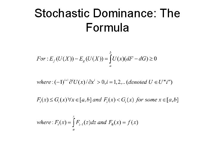
Stochastic Dominance: The Game • First developed in the finance literature as criteria for portfolio choice, transplanted to welfare by Atkinson, Kolm, Foster and Shorrocks • Working with “felicity” function U(x) where x is continuously defined over the range [a, b]. • Two alternative states defined by pdf’s f(x) and g(x) describing the distribution of x across agents. • Address the issue: “which state is preferred if the objective is E(U(x))? ” • Arrive at necessary and sufficient conditions (the stochastic dominance criteria)

Stochastic Dominance: The Formula

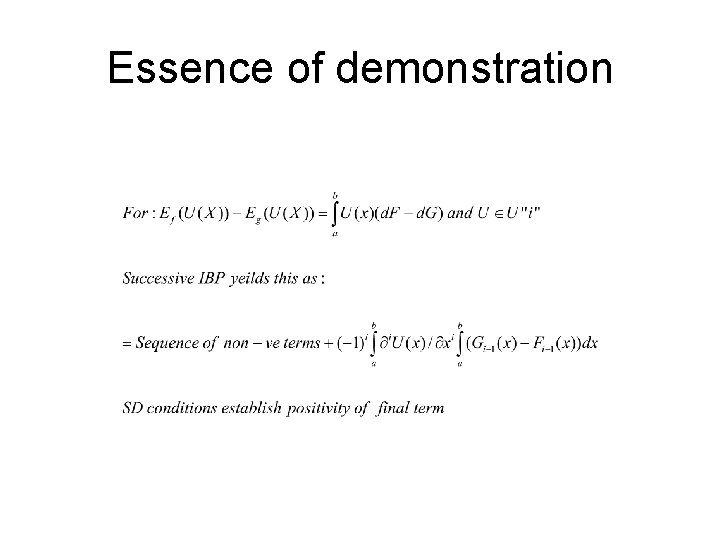
Essence of demonstration

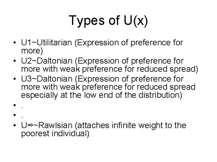
Types of U(x) • U 1~Utilitarian (Expression of preference for more) • U 2~Daltonian (Expression of preference for more with weak preference for reduced spread) • U 3~Daltonian (Expression of preference for more with weak preference for reduced spread especially at the low end of the distribution) • . • U∞~Rawlsian (attaches infinite weight to the poorest individual)

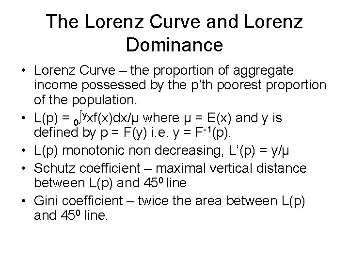
The Lorenz Curve and Lorenz Dominance • Lorenz Curve – the proportion of aggregate income possessed by the p’th poorest proportion of the population. • L(p) = 0∫yxf(x)dx/μ where μ = E(x) and y is defined by p = F(y) i. e. y = F-1(p). • L(p) monotonic non decreasing, L’(p) = y/μ • Schutz coefficient – maximal vertical distance between L(p) and 450 line • Gini coefficient – twice the area between L(p) and 450 line.

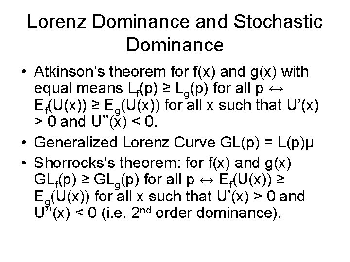
Lorenz Dominance and Stochastic Dominance • Atkinson’s theorem for f(x) and g(x) with equal means Lf(p) ≥ Lg(p) for all p ↔ Ef(U(x)) ≥ Eg(U(x)) for all x such that U’(x) > 0 and U’’(x) < 0. • Generalized Lorenz Curve GL(p) = L(p)μ • Shorrocks’s theorem: for f(x) and g(x) GLf(p) ≥ GLg(p) for all p ↔ Ef(U(x)) ≥ Eg(U(x)) for all x such that U’(x) > 0 and U’’(x) < 0 (i. e. 2 nd order dominance).

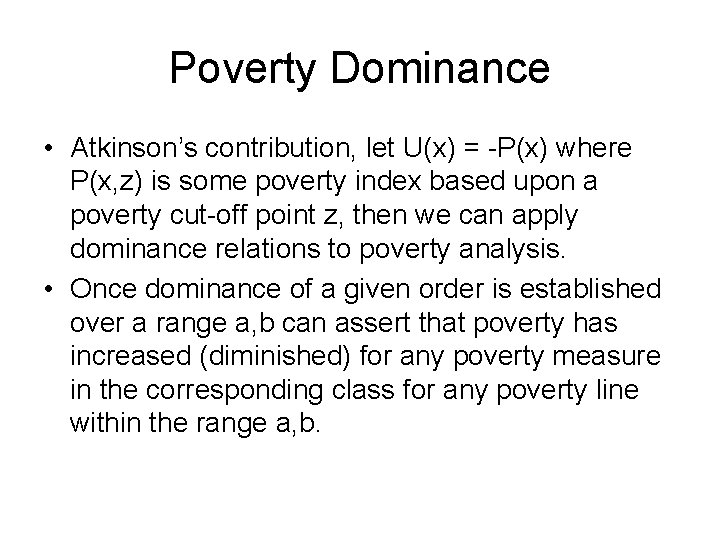
Poverty Dominance • Atkinson’s contribution, let U(x) = -P(x) where P(x, z) is some poverty index based upon a poverty cut-off point z, then we can apply dominance relations to poverty analysis. • Once dominance of a given order is established over a range a, b can assert that poverty has increased (diminished) for any poverty measure in the corresponding class for any poverty line within the range a, b.

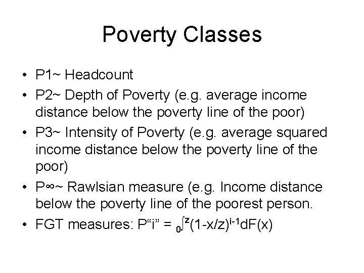
Poverty Classes • P 1~ Headcount • P 2~ Depth of Poverty (e. g. average income distance below the poverty line of the poor) • P 3~ Intensity of Poverty (e. g. average squared income distance below the poverty line of the poor) • P∞~ Rawlsian measure (e. g. Income distance below the poverty line of the poorest person. • FGT measures: P“i” = 0∫z(1 -x/z)i-1 d. F(x)

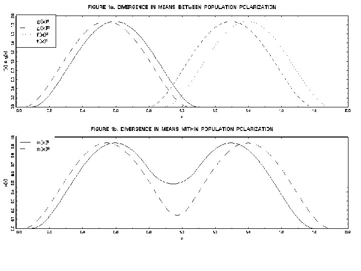
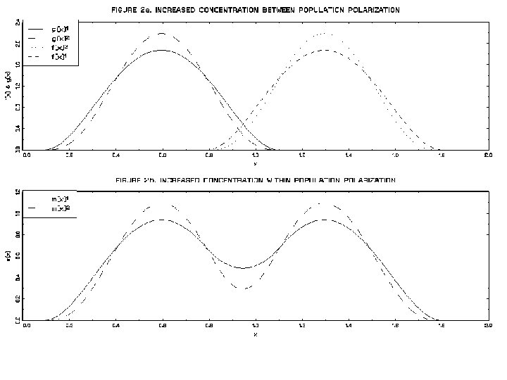
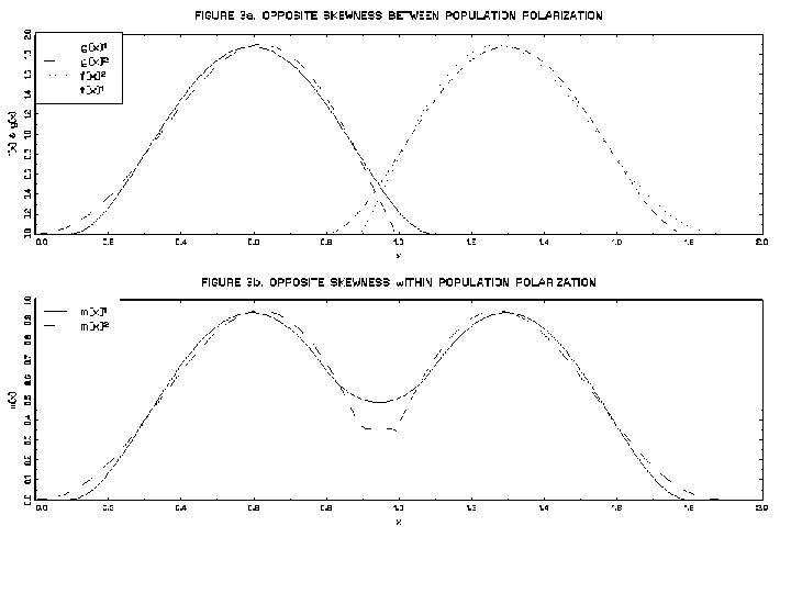
Polarization: Dominance as a measure of separation. • Dominance relationships can be used to categorize types of polarization.

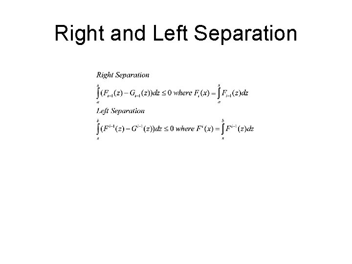
Polarization, Stochastic Dominance and Distributional Overlap • Polarization indices have been based upon a so-called Identification-Alienation nexus wherein notions of polarization are fostered jointly by an agent’s sense of increasing within-group identity and between-group distance or alienation. • The anatomy of polarization is best understood by employing ideas of “separation” drawn from the Stochastic Dominance Literature. • Various combinations of “separation” influence the degree to which distributions overlap. Can use an overlap measure as an indicator of potential polarizing states. • Advantage of great simplification in multivariate problems.

Right and Left Separation

Polarization and Stochastic Dominance

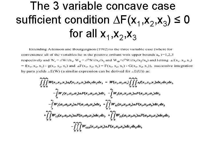
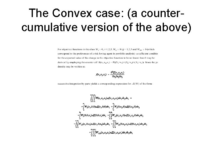
Multivariate Considerations • Atkinson and Bourguignon extended SD techniques to more than one dimension (2). • Life gets much more complicated here both theoretically (largely due to the conditions for concavity and convexity in multidimensional functions are much more complicated) and for empirical practicality reasons (curse of dimensionality).

The 3 variable concave case sufficient condition ∆F(x 1, x 2, x 3) ≤ 0 for all x 1, x 2, x 3

The Convex case: (a countercumulative version of the above)