Domain decomposition in parallel computing Ashok Srinivasan www

Domain decomposition in parallel computing Ashok Srinivasan www. cs. fsu. edu/~asriniva Florida State University

Outline • Background • Geometric partitioning • Graph partitioning – Static – Dynamic

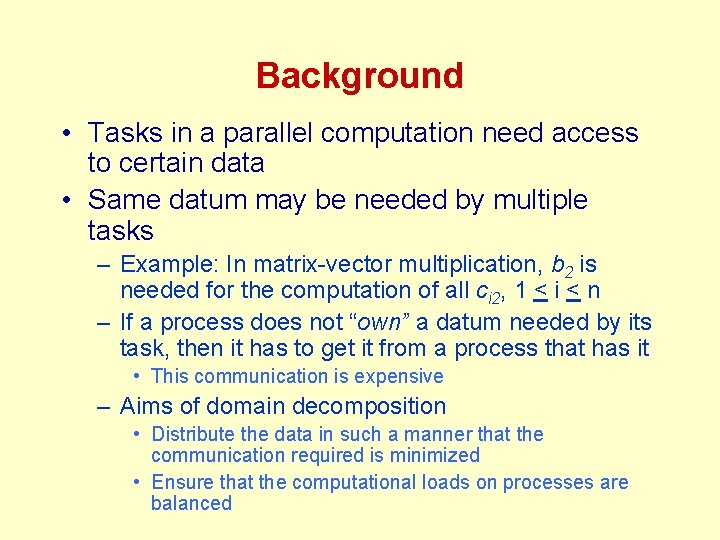
Background • Tasks in a parallel computation need access to certain data • Same datum may be needed by multiple tasks – Example: In matrix-vector multiplication, b 2 is needed for the computation of all ci 2, 1 < i < n – If a process does not “own” a datum needed by its task, then it has to get it from a process that has it • This communication is expensive – Aims of domain decomposition • Distribute the data in such a manner that the communication required is minimized • Ensure that the computational loads on processes are balanced

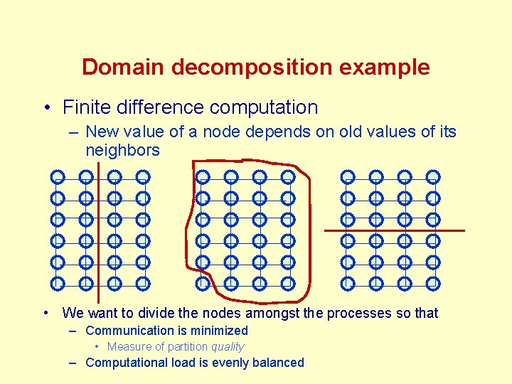
Domain decomposition example • Finite difference computation – New value of a node depends on old values of its neighbors • We want to divide the nodes amongst the processes so that – Communication is minimized • Measure of partition quality – Computational load is evenly balanced

Geometric partitioning • Partition a set of points – Uses only coordinate information • Balances the load – The heuristic tries to ensure that communication costs are low • Algorithms are typically fast, but partition not of high quality • Examples – Orthogonal recursive bisection – Inertial – Space filling curves

Orthogonal recursive bisection • Recursively bisect orthogonal to the longest dimension – Assume communication is proportional to the surface area of the domain – Recursive bisection • Divide into two pieces, keeping load balanced • Apply recursively, until desired number of partitions obtained

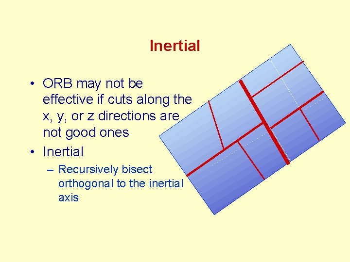
Inertial • ORB may not be effective if cuts along the x, y, or z directions are not good ones • Inertial – Recursively bisect orthogonal to the inertial axis

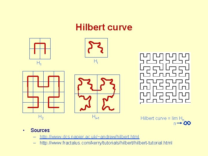
Space filling curves • Space filling curves – A continuous curve that fills the space – Order the points based on their relative position on the curve – Choose a curve that preserves proximity • Points that are close in space should be close in the ordering too • Example – Hilbert curve

Hilbert curve H 1 H 2 • Hi Hi+1 Hilbert curve = lim Hn n Sources – http: //www. dcs. napier. ac. uk/~andrew/hilbert. html – http: //www. fractalus. com/kerry/tutorials/hilbert-tutorial. html

Domain decomposition with a space filling curve • Order points based on their position on the curve • Divide into P parts – P is the number of processes • Space filling curves can be used in adaptive computations too • They can be extended to higher dimensions too

Graph partitioning • Model as graph partitioning – Graph G = (V, E) – Each task is represented by a vertex • A weight can be used to represent the computational effort – An edge exists between tasks if one needs data owned by the other • Weights can be associated with edges too – Goal • Partition vertices into P parts such that each partition has equal vertex weights • Minimize the weights of edges cut • Problem is NP complete – Edge cut metric • Judge the quality of the partitioning by the number of edges cut

Static graph partitioning • Combinatorial – Levelized nested dissection – Kernighan-Lin/Feduccia-Matheyses • Spectral partitioning • Multi-level methods

Combinatorial partitioning • Use only connectivity information • Examples – Levelized nested dissection – Kernighan-Lin/Feduccia-Matheyses

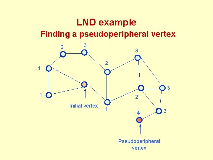
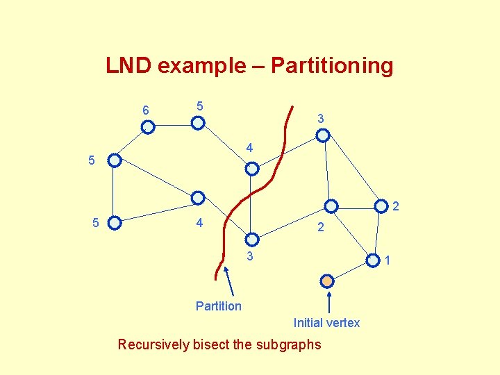
Levelized nested dissection (LND) • Idea is similar to the geometric methods – But cannot use coordinate information – Instead of projecting vertices along the longest axis, order them based on distance from a vertex that may be one extreme of the longest dimension of a graph • Pseudo-peripheral vertex – Perform a breadth-first search, starting from an arbitrary vertex – The vertex that is encountered last might be a good approximation to a peripheral vertex

LND example Finding a pseudoperipheral vertex 2 3 3 2 1 3 1 2 Initial vertex 1 4 Pseudoperipheral vertex 3

LND example – Partitioning 6 5 3 4 5 2 5 4 2 3 1 Partition Initial vertex Recursively bisect the subgraphs

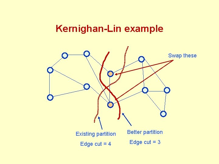
Kernighan-Lin/Fiduccia-Matheyses • Refines an existing partition • Kernighan-Lin – Consider pairs of vertices from different partitions – Choose a pair whose swapping will result in the best improvement in partition quality • The best improvement may actually be a worsening – Perform several passes • Choose best partition among those encountered • Fiduccia-Matheyses – Similar but more efficient • Boundary Kernighan-Lin – Consider only boundary vertices to swap • . . . and many other variants

Kernighan-Lin example Swap these Existing partition Better partition Edge cut = 4 Edge cut = 3

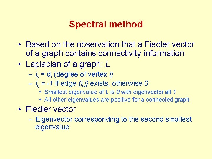
Spectral method • Based on the observation that a Fiedler vector of a graph contains connectivity information • Laplacian of a graph: L – lii = di (degree of vertex i) – lij = -1 if edge {i, j} exists, otherwise 0 • Smallest eigenvalue of L is 0 with eigenvector all 1 • All other eigenvalues are positive for a connected graph • Fiedler vector – Eigenvector corresponding to the second smallest eigenvalue

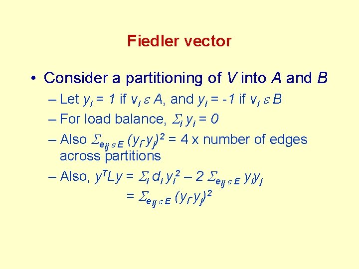
Fiedler vector • Consider a partitioning of V into A and B – Let yi = 1 if vi e A, and yi = -1 if vi e B – For load balance, Si yi = 0 – Also Seij e E (yi-yj)2 = 4 x number of edges across partitions – Also, y. TLy = Si di yi 2 – 2 Seij e E yiyj = Seij e E (yi-yj)2

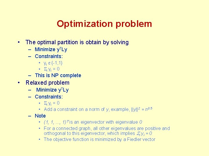
Optimization problem • The optimal partition is obtain by solving – Minimize y. TLy – Constraints: • yi e {-1, 1} • Si yi = 0 – This is NP complete • Relaxed problem – Minimize y. TLy – Constraints: • Si yi = 0 • Add a constraint on a norm of y, example, ||y||2 = n 0. 5 – Note • (1, 1, . . . , 1)T is an eigenvector with eigenvalue 0 • For a connected graph, all other eigenvalues are positive and orthogonal to this eigenvector, which implies Si yi = 0 • The objective function is minimized by a Fiedler vector

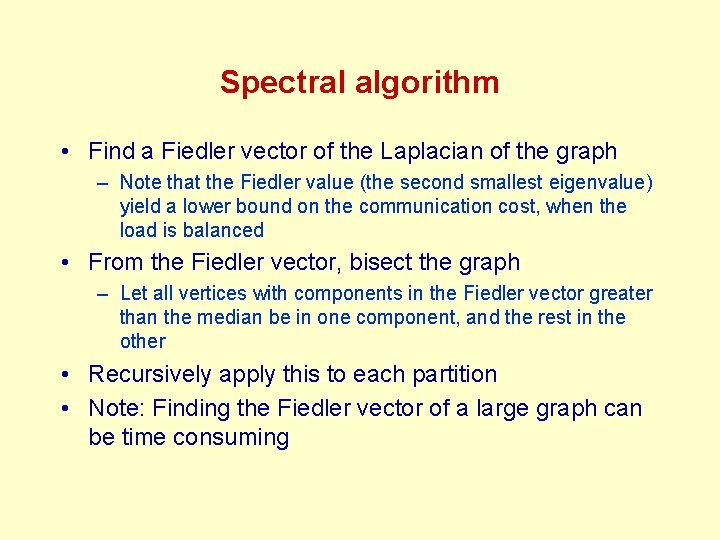
Spectral algorithm • Find a Fiedler vector of the Laplacian of the graph – Note that the Fiedler value (the second smallest eigenvalue) yield a lower bound on the communication cost, when the load is balanced • From the Fiedler vector, bisect the graph – Let all vertices with components in the Fiedler vector greater than the median be in one component, and the rest in the other • Recursively apply this to each partition • Note: Finding the Fiedler vector of a large graph can be time consuming

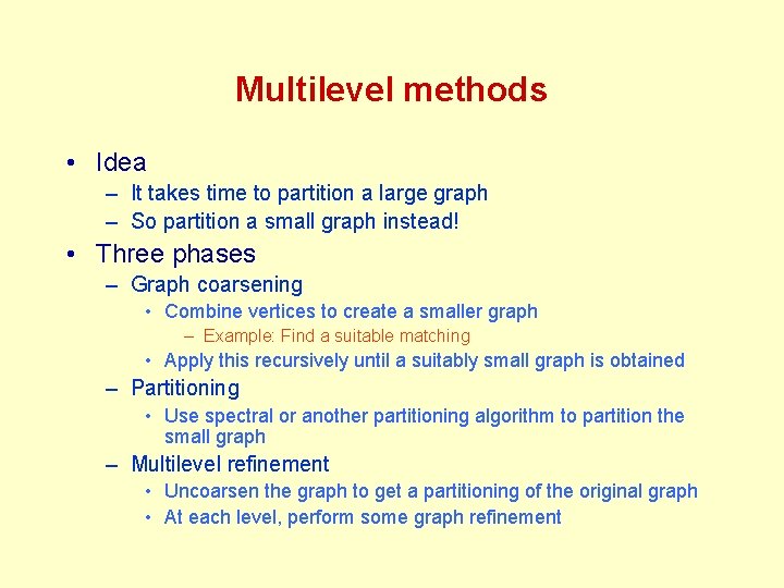
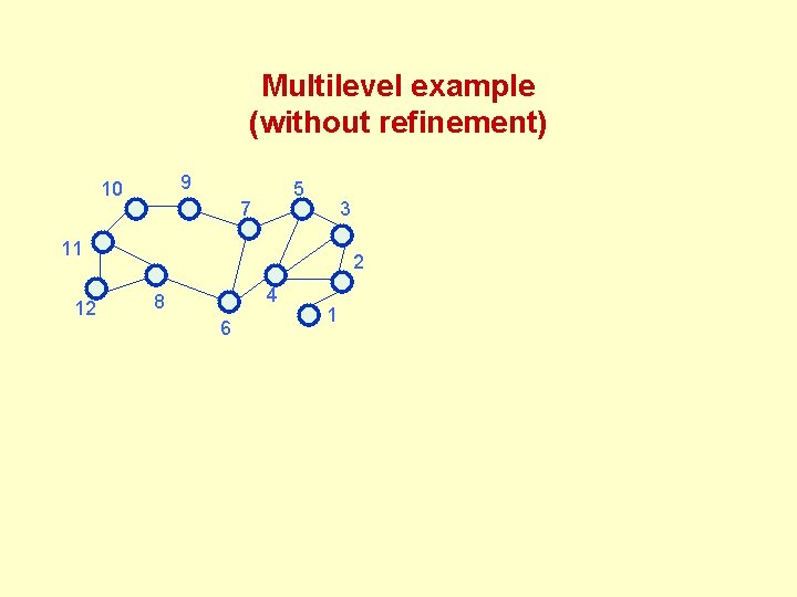
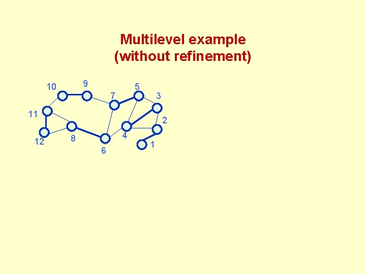
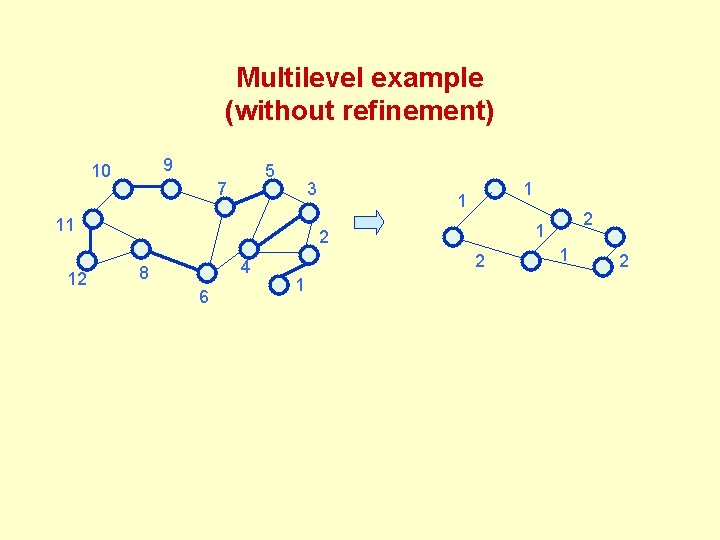
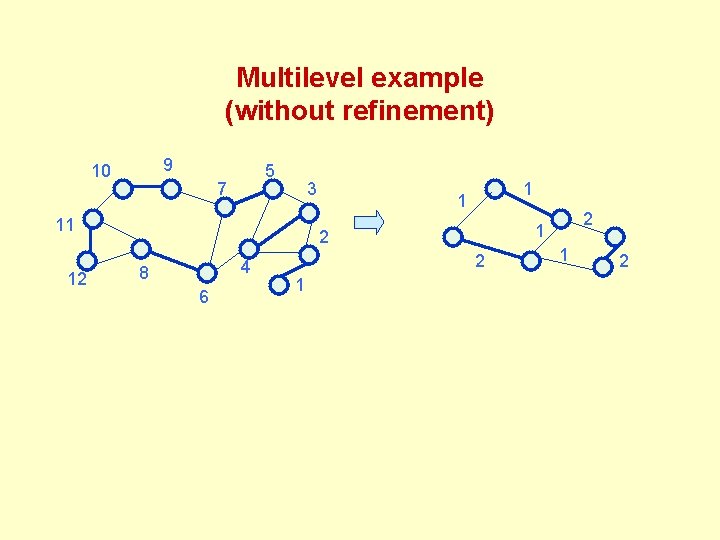
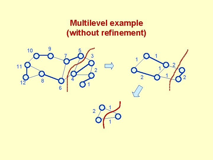
Multilevel methods • Idea – It takes time to partition a large graph – So partition a small graph instead! • Three phases – Graph coarsening • Combine vertices to create a smaller graph – Example: Find a suitable matching • Apply this recursively until a suitably small graph is obtained – Partitioning • Use spectral or another partitioning algorithm to partition the small graph – Multilevel refinement • Uncoarsen the graph to get a partitioning of the original graph • At each level, perform some graph refinement

Multilevel example (without refinement) 9 10 5 7 3 11 12 2 4 8 6 1

Multilevel example (without refinement) 9 10 5 7 3 11 12 2 4 8 6 1

Multilevel example (without refinement) 9 10 5 7 3 11 12 1 1 2 4 8 6 2 1 1 2

Multilevel example (without refinement) 9 10 5 7 3 11 12 1 1 2 4 8 6 2 1 1 2

Multilevel example (without refinement) 9 10 5 7 3 11 12 1 1 2 4 8 6 2 1 2 2 1 1 2

Dynamic partitioning • We have an initial partitioning – Now, the graph changes – Determine a good partition, fast – Also minimize the number of vertices that need to be moved • Examples – PLUM – Jostle

PLUM • Partition based on the initial mesh – Vertex and edge weights alone changed • Map partitions to processors – Use more partitions than processors • Ensures finer granularity – Compute a similarity matrix • Measures savings on data redistribution cost for each (processor, partition) pair • Choose assignment of partitions to processors – Example: Maximum weight matching » Duplicate each processor: # of partitions/P times – Alternative: Greedy approximation algorithm • http: //citeseer. nj. nec. com/oliker 98 plum. html

JOSTLE • Use Hu and Blake’s diffusive scheme for load balancing – Solve Lx = b • L = Laplacian, bi = Weight on process Pi – Average weight – Move max(xi-xj, 0) weight between Pi and Pj • Select vertices to move, based on relative gain • http: //citeseer. nj. nec. com/walshaw 97 parallel. html