Doing Bayesian Data Analysis with R and JAGS

Doing Bayesian Data Analysis with R and JAGS Examples from Kruschke text Darrell A. Worthy Texas A&M

Download the latest version of R • This tutorial was written with R version 3. 4. • You can download it here https: //cran. rstudio. com/ • Also download the latest version of Rstudio https: //www. rstudio. com/products/rstudio/download 2/ • Download JAGS at: https: //sourceforge. net/projects/mcmcjags/? source=typ_redirect • Once JAGS is installed, invoke Rstudio, and on the command line type: install. packages(“rjags”) and install. packages(“runjags”)

Setting default working directory in R • This is optional but I will set the default working directory as the folder DBDA 2 EPrograms folder, since that is what we will be working on. • The other option is to use the setwd() function • Click on Tools, then Global Options, then under Default Working Directory. • Click Browse and navigate to the DBDA 2 EPrograms, click Select Folder and then Apply.

Stan • Kruschke uses JAGS and Stan to do much of the same analyses. • Due to the short nature of this course and Stan’s somewhat intensive installation process I will just be showing a few examples using JAGS. • Stan is the most cutting edge MCMC interface with RStan devoted to interfacing with Stan and Rstanarm devoted to taking many common R commands such as lm or glm and translating them into Bayesian analyses. • To download Rstan go to: https: //github. com/standev/rstan/wiki/RStan-Getting-Started. • You can then use Kruschke’s Stan code along with the JAGS code.

Regression using JAGS • We used JASP to analyze the Worthy, Byrne, & Fields (2014) data on worry predicting decision-making behavior more than anxiety and mood. • One thing we did not get from JASP were regression coefficients. • We might like to report these and want to do so without having to use point estimates from OLS analysis. • JASP allows us to test hypotheses and we got clear evidence that worry was the biggest and only predictor. • However, if we have more applied goals we might want to examine the posterior distributions for our Regression coefficients. • JASP also did not directly tell us R 2 values, and these analyses will give us something similar.

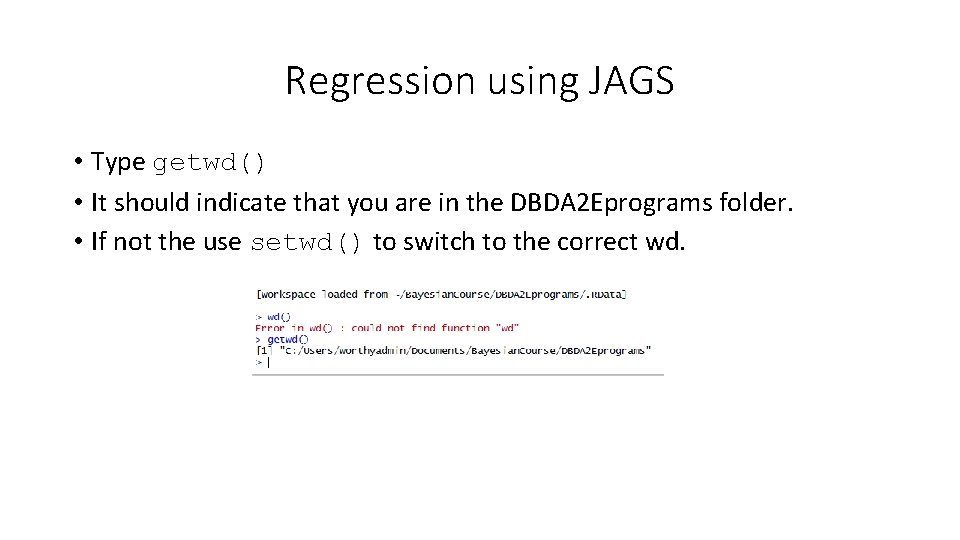
Regression using JAGS • Type getwd() • It should indicate that you are in the DBDA 2 Eprograms folder. • If not the use setwd() to switch to the correct wd.

Regression using JAGS • In Chapter 18 of the Kruschke text there is an example on multiple regression using two predictors. • The data come from Guber 1999; the DV is the average total SAT score per state, the predictors are amount spent per pupil on SAT instruction, and the % of students taking the test. • Amount spent is negatively correlated with SAT scores, but this is because amount spent is correlated with % of students taking the test. • This negative correlation for amount spent might lead some people to argue against public spending for education. • As more mediocre students are encouraged to take the SAT scores drop, therefore the % of students taking the test could be the underlying cause.

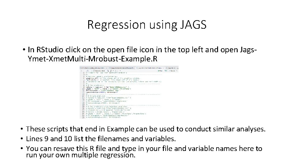
Regression using JAGS • In RStudio click on the open file icon in the top left and open Jags. Ymet-Xmet. Multi-Mrobust-Example. R • These scripts that end in Example can be used to conduct similar analyses. • Lines 9 and 10 list the filenames and variables. • You can resave this R file and type in your file and variable names here to run your own multiple regression.

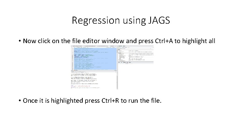
Regression using JAGS • Now click on the file editor window and press Ctrl+A to highlight all • Once it is highlighted press Ctrl+R to run the file.

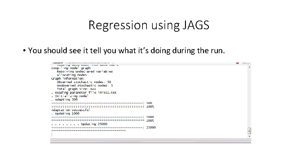
Regression using JAGS • You should see it tell you what it’s doing during the run.

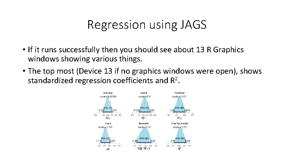
Regression using JAGS • If it runs successfully then you should see about 13 R Graphics windows showing various things. • The top most (Device 13 if no graphics windows were open), shows standardized regression coefficients and R 2.

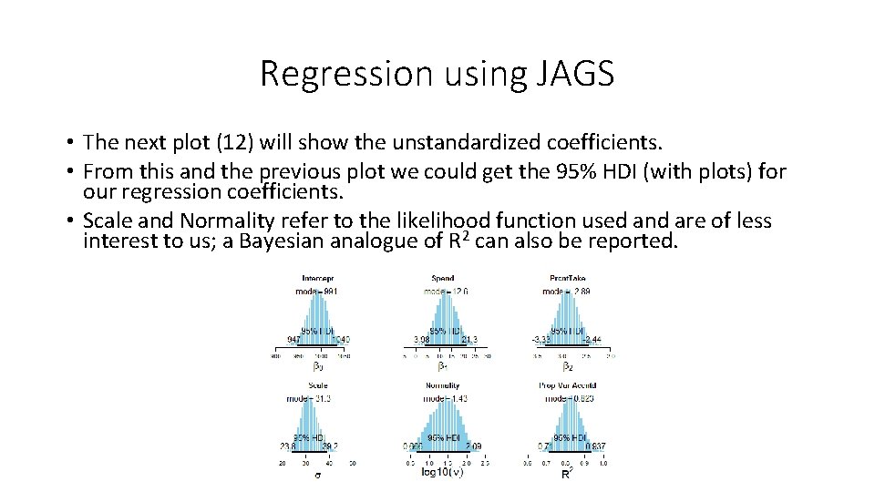
Regression using JAGS • The next plot (12) will show the unstandardized coefficients. • From this and the previous plot we could get the 95% HDI (with plots) for our regression coefficients. • Scale and Normality refer to the likelihood function used and are of less interest to us; a Bayesian analogue of R 2 can also be reported.

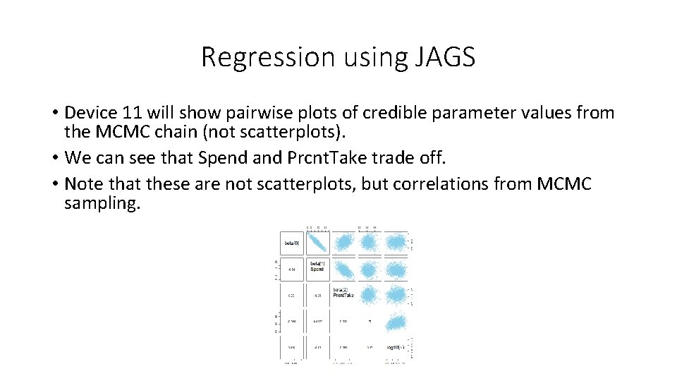
Regression using JAGS • Device 11 will show pairwise plots of credible parameter values from the MCMC chain (not scatterplots). • We can see that Spend and Prcnt. Take trade off. • Note that these are not scatterplots, but correlations from MCMC sampling.

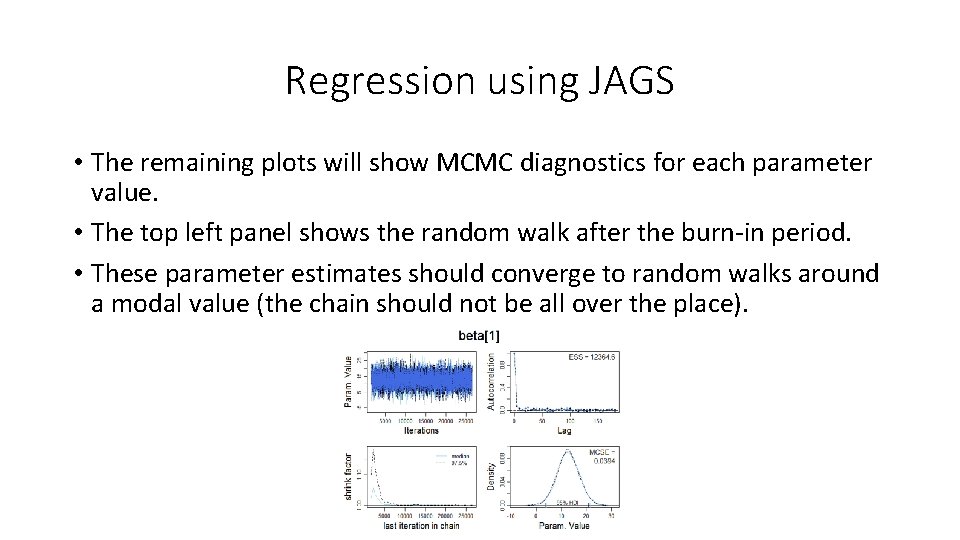
Regression using JAGS • The remaining plots will show MCMC diagnostics for each parameter value. • The top left panel shows the random walk after the burn-in period. • These parameter estimates should converge to random walks around a modal value (the chain should not be all over the place).

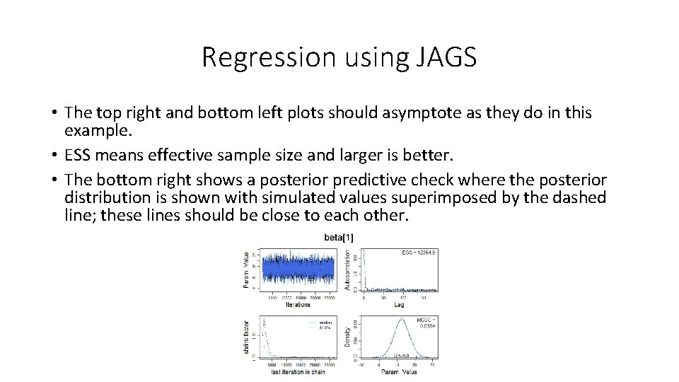
Regression using JAGS • The top right and bottom left plots should asymptote as they do in this example. • ESS means effective sample size and larger is better. • The bottom right shows a posterior predictive check where the posterior distribution is shown with simulated values superimposed by the dashed line; these lines should be close to each other.

Regression using JAGS • These high level scripts that end in Example can be modified to run your data. • In Rstudio open Jags-Ymet-XMet. Multi-Robust. Worthy. Byrne. Fields 2014. R • I made this file by saving Jags-Ymet-Xmet. Multi-Robust-Example. R with a different name that included my data. • I then modified the data file and variable names and saved. • (in computer programming it’s usually faster to start from an existing file than from scratch). • Note that your variable names in your. csv file cannot have any spaces.

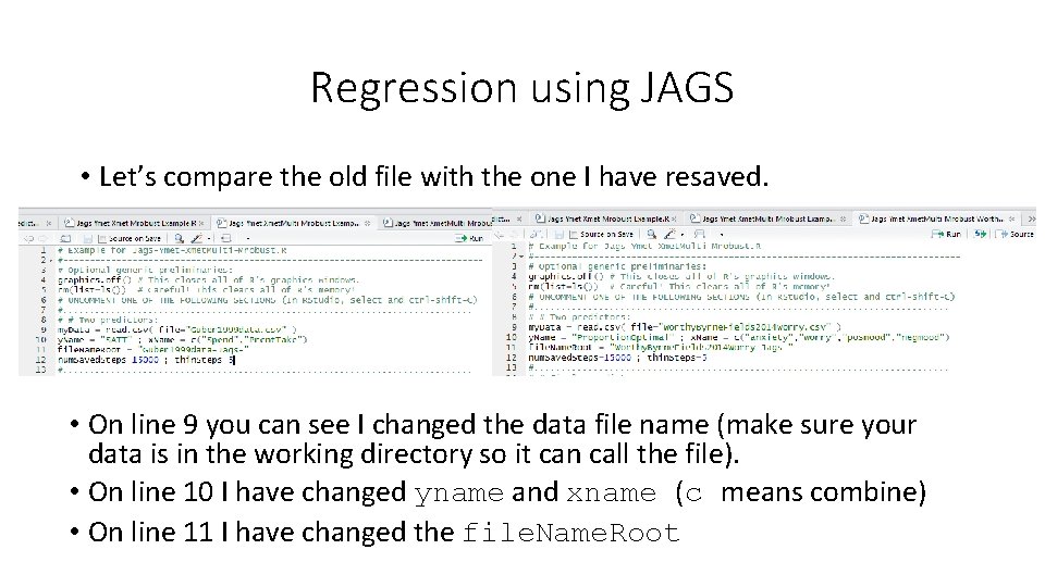
Regression using JAGS • Let’s compare the old file with the one I have resaved. • On line 9 you can see I changed the data file name (make sure your data is in the working directory so it can call the file). • On line 10 I have changed yname and xname (c means combine) • On line 11 I have changed the file. Name. Root

Regression using JAGS • Now let’s press CTRL+A and CTRL+R to see if we can run the analyses on this data set. • You should get about 19 R Graphics device windows this time. • You can see the standardized coefficients; how many parameters have 95% HDIs well away from zero?

Summary • I highly recommend the Kruschke text if you think you would like to start conducting Bayesian data analyses. • Chapters 16 -24 cover examples using different types of data that cover all the analyses you have learned about in ANOVA and Regression courses as well as some more advanced topics. • My recommended practice is to report Bayes factors using JASP as alternatives to NHST. • Use R and Jags (or Stan) to provide additional data on particular parameter estimates that are not currently available with JASP. • We’ve seen how easy it is to use R and JAGS, and it’s worth a little extra analysis for a paper that will be in the published literature forever. • Arguably JAGS is more necessary for regression with metric predictors than for ANOVA since we do not normally use coefficients to describe main effects or interactions.

Regression using JAGS • Now it’s time to try some Bayesian data analysis on your own data! • I recommend first analyzing them with JASP and then possibly trying to resave and modify the Jags example file that best fits your data. • JAGS files start with specifying the scale of the y variable (binom, count, dich, met (metric), nom (nominal), ordinal). • They then specify the scale of the x variable(s) and how many variables there are. • The files ending in Example are the ones you want to use. • If you run into problems first try to resolve it on your own as that will better help you learn than someone giving you the answer.