Do Now Find the cube roots of 8

Do Now Find the cube roots of 8 1

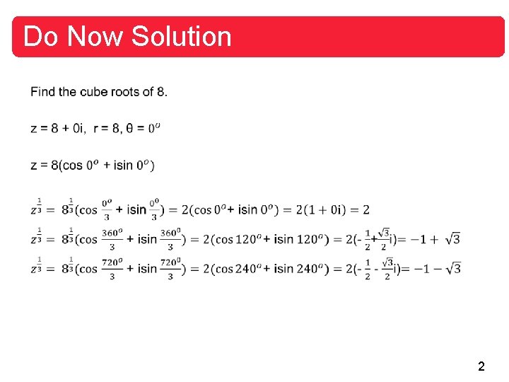
Do Now Solution 2

Parametric Equations 3

Objectives Evaluate sets of parametric equations for given values of the parameter. Sketch curves that are represented by sets of parametric equations. Rewrite sets of parametric equations as single rectangular equations by eliminating the parameter. Find sets of parametric equations for graphs. 4

Plane Curves 5

Plane Curves Up to this point you have been representing a graph by a single equation involving two variables such as x and y. In this section, you will study situations in which it is useful to introduce a third variable to represent a curve in the plane. To see the usefulness of this procedure, consider the path of an object that is propelled into the air at an angle of 45. 6

Plane Curves When the initial velocity of the object is 48 feet per second, it can be shown that the object follows the parabolic path Rectangular equation 7

Plane Curves However, this equation does not tell the whole story. Although it does tell you where the object has been, it does not tell you when the object was at a given point (x, y) on the path. To determine this time, you can introduce a third variable t, called a parameter. It is possible to write both x and y as functions of t to obtain the parametric equations x = 24 y = – 16 t 2 + 24 Parametric equation for x . Parametric equation for y 8

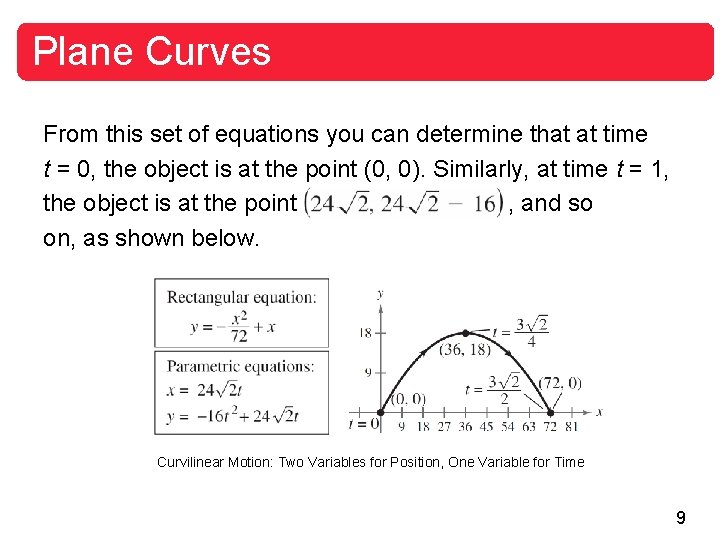
Plane Curves From this set of equations you can determine that at time t = 0, the object is at the point (0, 0). Similarly, at time t = 1, the object is at the point , and so on, as shown below. Curvilinear Motion: Two Variables for Position, One Variable for Time 9

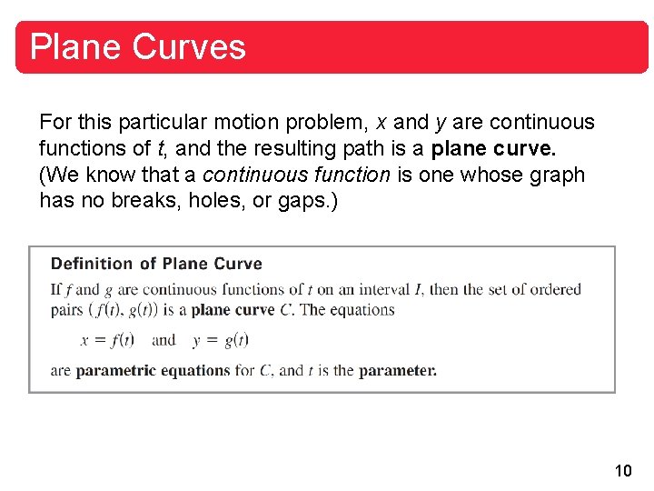
Plane Curves For this particular motion problem, x and y are continuous functions of t, and the resulting path is a plane curve. (We know that a continuous function is one whose graph has no breaks, holes, or gaps. ) 10

Sketching a Plane Curve 11

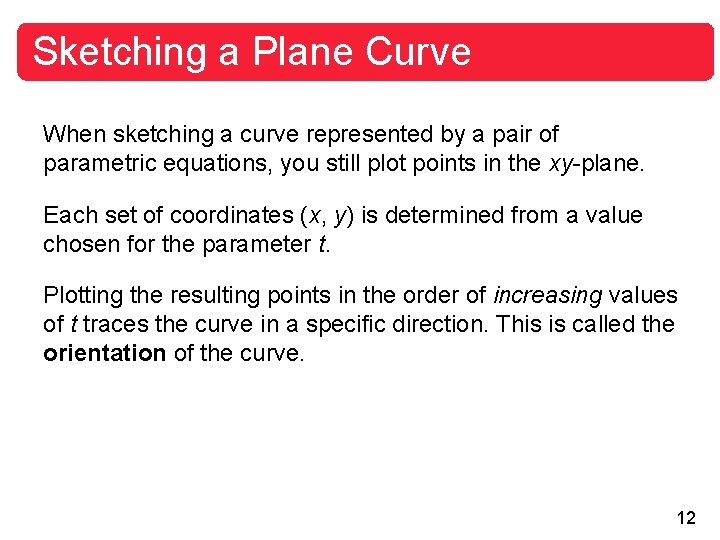
Sketching a Plane Curve When sketching a curve represented by a pair of parametric equations, you still plot points in the xy-plane. Each set of coordinates (x, y) is determined from a value chosen for the parameter t. Plotting the resulting points in the order of increasing values of t traces the curve in a specific direction. This is called the orientation of the curve. 12

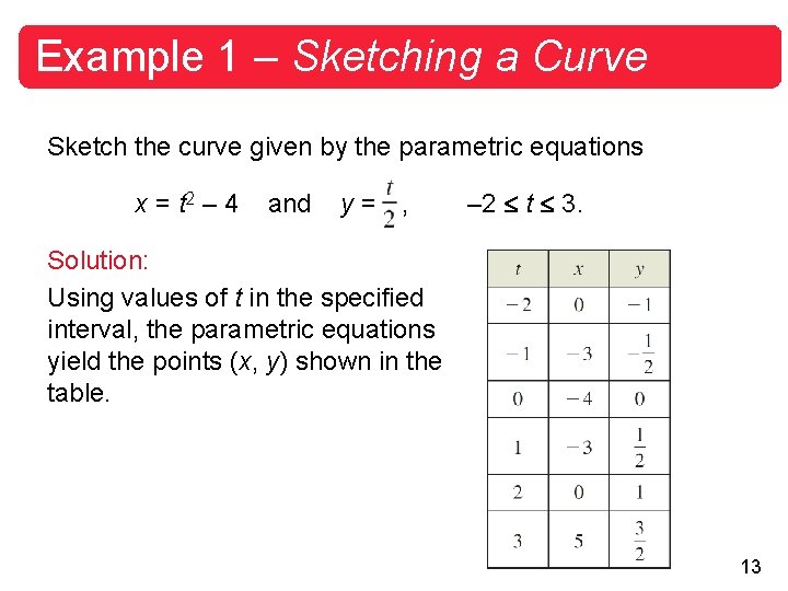
Example 1 – Sketching a Curve Sketch the curve given by the parametric equations x = t 2 – 4 and y= , – 2 t 3. Solution: Using values of t in the specified interval, the parametric equations yield the points (x, y) shown in the table. 13

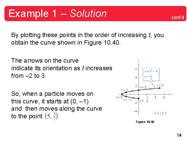
Example 1 – Solution cont’d By plotting these points in the order of increasing t, you obtain the curve shown in Figure 10. 40. The arrows on the curve indicate its orientation as t increases from – 2 to 3. So, when a particle moves on this curve, it starts at (0, – 1) and then moves along the curve to the point. Figure 10. 40 14

Sketching a Plane Curve Note that the graph shown in Figure 10. 40 does not define y as a function of x. This points out one benefit of parametric equations—they can be used to represent graphs that are more general than graphs of functions. Two different sets of parametric equations can have the same graph. For example, the set of parametric equations x = 4 t 2 – 4 and y = t, – 1 t has the same graph as the set of parametric equations given in Example 1. 15

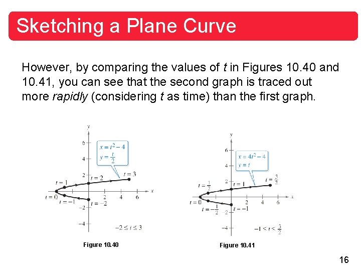
Sketching a Plane Curve However, by comparing the values of t in Figures 10. 40 and 10. 41, you can see that the second graph is traced out more rapidly (considering t as time) than the first graph. Figure 10. 40 Figure 10. 41 16

Sketching a Plane Curve So, in applications, different parametric representations can be used to represent various speeds at which objects travel along a given path. 17

Eliminating the Parameter 18

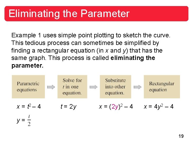
Eliminating the Parameter Example 1 uses simple point plotting to sketch the curve. This tedious process can sometimes be simplified by finding a rectangular equation (in x and y) that has the same graph. This process is called eliminating the parameter. x = t 2 – 4 t = 2 y x = (2 y)2 – 4 x = 4 y 2 – 4 y= 19

Eliminating the Parameter Now you can recognize that the equation x = 4 y 2 – 4 represents a parabola with a horizontal axis and vertex at (– 4, 0). When converting equations from parametric to rectangular form, you may need to alter the domain of the rectangular equation so that its graph matches the graph of the parametric equations. Such a situation is demonstrated in Example 2. 20

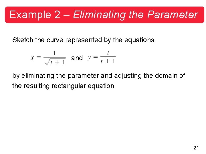
Example 2 – Eliminating the Parameter Sketch the curve represented by the equations and by eliminating the parameter and adjusting the domain of the resulting rectangular equation. 21

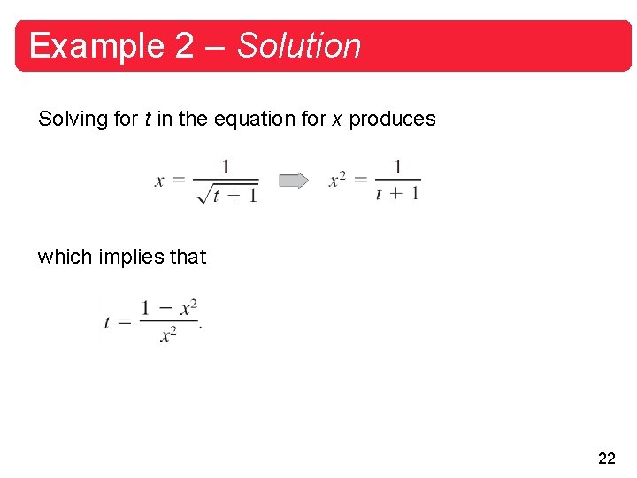
Example 2 – Solution Solving for t in the equation for x produces which implies that 22

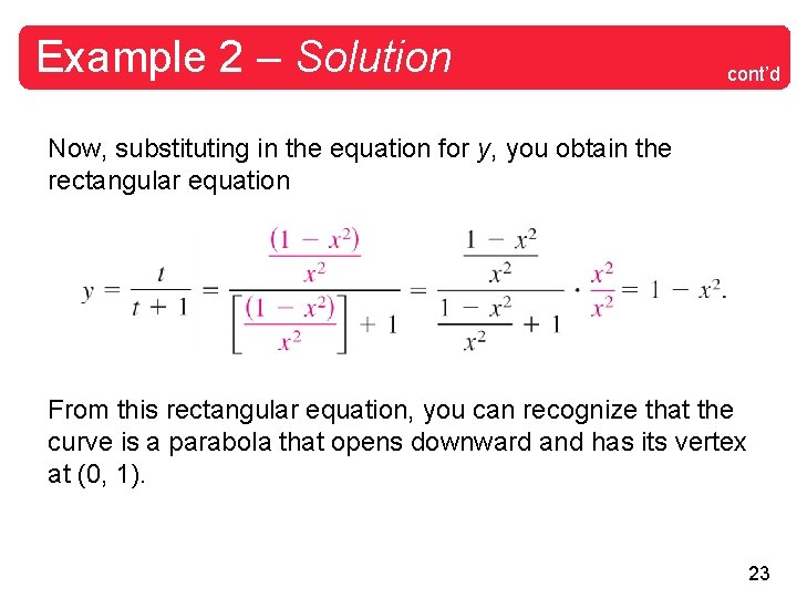
Example 2 – Solution cont’d Now, substituting in the equation for y, you obtain the rectangular equation From this rectangular equation, you can recognize that the curve is a parabola that opens downward and has its vertex at (0, 1). 23

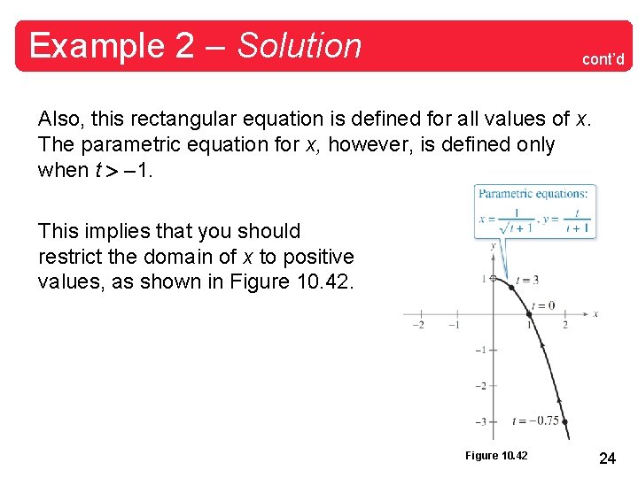
Example 2 – Solution cont’d Also, this rectangular equation is defined for all values of x. The parametric equation for x, however, is defined only when t – 1. This implies that you should restrict the domain of x to positive values, as shown in Figure 10. 42 24

Eliminating the Parameter In Example 2, it is important to realize that eliminating the parameter is primarily an aid to curve sketching. When the parametric equations represent the path of a moving object, the graph alone is not sufficient to describe the object’s motion. You still need the parametric equations to tell you the position, direction, and speed at a given time. 25

Finding Parametric Equations for a Graph 26

Finding Parametric Equations for a Graph You have been studying techniques for sketching the graph represented by a set of parametric equations. Now consider the reverse problem—that is, how can you find a set of parametric equations for a given graph or a given physical description? You know that such a representation is not unique. 27

Finding Parametric Equations for a Graph That is, the equations x = 4 t 2 – 4 and y = t, – 1 t produced the same graph as the equations x = t 2 – 4 and y = , – 2 t 3. This is further demonstrated in Example 4. 28

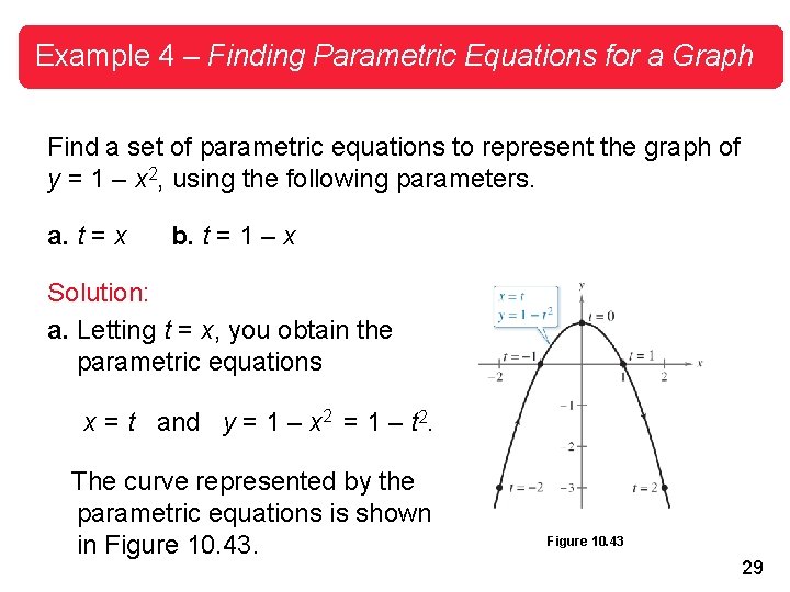
Example 4 – Finding Parametric Equations for a Graph Find a set of parametric equations to represent the graph of y = 1 – x 2, using the following parameters. a. t = x b. t = 1 – x Solution: a. Letting t = x, you obtain the parametric equations x = t and y = 1 – x 2 = 1 – t 2. The curve represented by the parametric equations is shown in Figure 10. 43 29

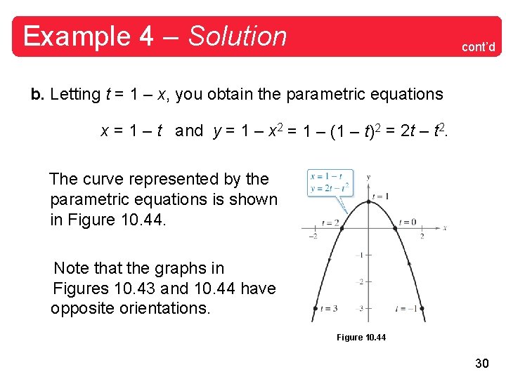
Example 4 – Solution cont’d b. Letting t = 1 – x, you obtain the parametric equations x = 1 – t and y = 1 – x 2 = 1 – (1 – t)2 = 2 t – t 2. The curve represented by the parametric equations is shown in Figure 10. 44. Note that the graphs in Figures 10. 43 and 10. 44 have opposite orientations. Figure 10. 44 30

Finding Parametric Equations for a Graph A cycloid is a curve traced out by a point P on a circle as the circle rolls along a straight line in a plane. 31

Example 5 – Parametric Equations for a Cycloid Write parametric equations for a cycloid traced out by a point P on a circle of radius a as the circle rolls along the x-axis given that P is at a minimum when x = 0. Solution: As the parameter, let be the measure of the circle’s rotation, and let the point P(x, y) begin at the origin. When = 0, P is at the origin; when = , P is at a maximum point ( a, 2 a); and when = 2 , P is back on the x-axis at (2 a, 0). 32

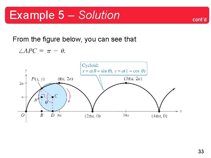
Example 5 – Solution cont’d From the figure below, you can see that 33

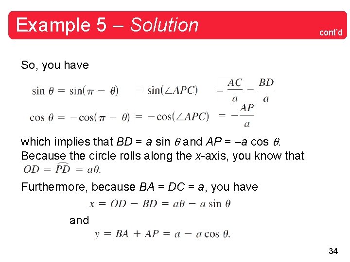
Example 5 – Solution cont’d So, you have which implies that BD = a sin and AP = –a cos . Because the circle rolls along the x-axis, you know that Furthermore, because BA = DC = a, you have and 34

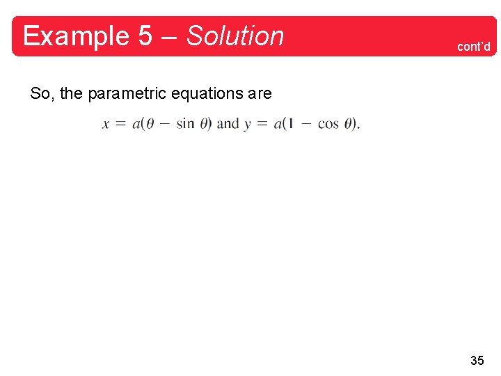
Example 5 – Solution cont’d So, the parametric equations are 35