Do D Sensor Processing Applications and Supporting Software

Do. D Sensor Processing: Applications and Supporting Software Technology Dr. Jeremy Kepner MIT Lincoln Laboratory This work is sponsored by the High Performance Computing Modernization Office under Air Force Contract F 19628 -00 -C-0002. Opinions, interpretations, conclusions, and recommendations are those of the author and are not necessarily endorsed by the Unites States Government. MIT Lincoln Laboratory Slide-1 SC 2002 Tutorial

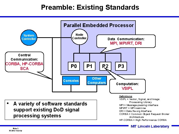
Preamble: Existing Standards Parallel Embedded Processor System Controller Node Controller Data Communication: MPI, MPI/RT, DRI Control Communication: CORBA, HP-CORBA SCA P 0 P 1 Consoles P 2 Other Computers P 3 Computation: VSIPL • A variety of software standards support existing Do. D signal processing systems Slide-2 SC 2002 Tutorial Definitions VSIPL = Vector, Signal, and Image Processing Library MPI = Message-passing interface MPI/RT = MPI real-time DRI = Data Re-org Interface CORBA = Common Object Request Broker Architecture HP-CORBA = High Performance CORBA MIT Lincoln Laboratory

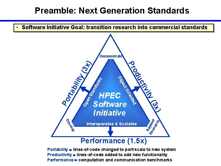
Preamble: Next Generation Standards • Software Initiative Goal: transition research into commercial standards (3 x Op en Sta nd ard s ity bil rta Po lop A Re pplie se d arc h ) ve De Interoperable & Scalable (3 x ted n rie HPEC Software Initiative ity tiv t. O jec Ob uc od Pr ) Demonstrate Performance (1. 5 x) Slide-3 SC 2002 Tutorial Portability lines-of-code changed to port/scale to new system Productivity lines-of-code added to add new functionality MIT Lincoln Laboratory Performance computation and communication benchmarks

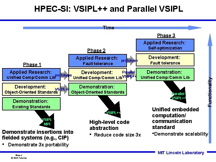
HPEC-SI: VSIPL++ and Parallel VSIPL Time Phase 3 Applied Research: Self-optimization Phase 2 Fault tolerance Phase 1 Applied Research: prototype Unified Comp/Comm Lib Development: VSIPL++ Object-Oriented Standards Development: prototype Fault tolerance Demonstration: Development: Parallel Unified Comp/Comm Lib. VSIPL++ Unified Comp/Comm Lib Demonstration: Object-Oriented Standards Demonstration: Existing Standards VSIPL++ VSIPL MPI Demonstrate insertions into fielded systems (e. g. , CIP) • High-level code abstraction • Reduce code size 3 x Parallel VSIPL++ Unified embedded computation/ communication standard • Demonstrate scalability Demonstrate 3 x portability Slide-4 SC 2002 Tutorial Functionality Applied Research: MIT Lincoln Laboratory

Preamble: The Links High Performance Embedded Computing Workshop http: //www. ll. mit. edu/HPEC High Performance Embedded Computing Software Initiative http: //www. hpec-si. org/ Vector, Signal, and Image Processing Library http: //www. vsipl. org/ MPI Software Technologies, Inc. http: //www. mpi-softtech. com/ Data Reorganization Initiative http: //www. data-re. org/ Code. Sourcery, LLC http: //www. codesourcery. com/ Matlab. MPI http: //www. ll. mit. edu/Matlab. MPI MIT Lincoln Laboratory Slide-5 SC 2002 Tutorial

Outline • Introduction • Processing Algorithms • Parallel System Analysis • Software Frameworks • Summary Slide-6 SC 2002 Tutorial • Do. D Needs • Parallel Stream Computing • Basic Pipeline Processing MIT Lincoln Laboratory

Why Is Do. D Concerned with Embedded Software? Source: “HPEC Market Study” March 2001 Estimated Do. D expenditures for embedded signal and image processing hardware and software ($B) • COTS acquisition practices have shifted the burden from “point design” hardware to “point design” software (i. e. COTS HW requires COTS SW) • Software costs for embedded systems could be reduced by one-third with improved programming models, methodologies, and standards Slide-7 SC 2002 Tutorial MIT Lincoln Laboratory

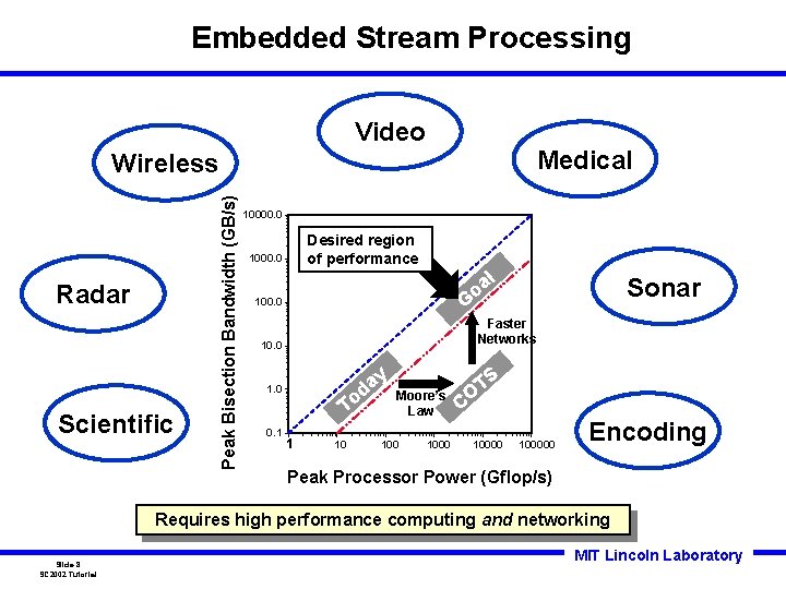
Embedded Stream Processing Video Medical Radar Scientific Peak Bisection Bandwidth (GB/s) Wireless 10000. 0 Desired region of performance 1000. 0 l a o Faster Networks 10. 0 y a d 1. 0 0. 1 Sonar G 100. 0 To 1 10 Moore’s Law 1000 TS CO 100000 Encoding Peak Processor Power (Gflop/s) Requires high performance computing and networking Slide-8 SC 2002 Tutorial MIT Lincoln Laboratory

Military Embedded Processing REQUIREMENTS INCREASING BY AN ORDER OF MAGNITUDE EVERY 5 YEARS EMBEDDED PROCESSING REQUIREMENTS WILL EXCEED 10 TFLOPS IN THE 2005 -2010 TIME FRAME Slide-9 SC 2002 Tutorial MIT Lincoln Laboratory Signal processing drives computing requirements

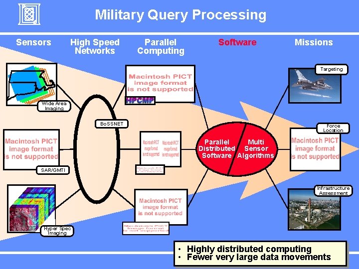
Military Query Processing Sensors High Speed Networks Parallel Computing Software Missions Targeting Wide Area Imaging Bo. SSNET Force Location Parallel Multi Distributed Sensor Software Algorithms SAR/GMTI Infrastructure Assessment Hyper Spec Imaging Slide-10 SC 2002 Tutorial • Highly distributed. MIT computing Laboratory • Fewer very large data. Lincoln movements

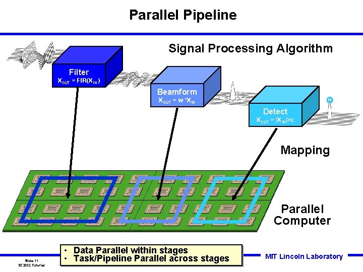
Parallel Pipeline Signal Processing Algorithm Filter XOUT = FIR(XIN ) Beamform XOUT = w *XIN Detect XOUT = |XIN|>c Mapping Parallel Computer Slide-11 SC 2002 Tutorial • Data Parallel within stages • Task/Pipeline Parallel across stages MIT Lincoln Laboratory

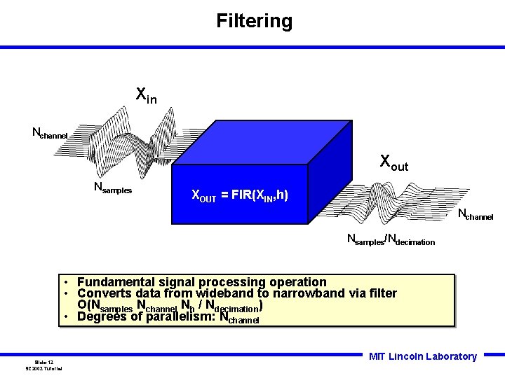
Filtering Xin Nchannel Xout Nsamples XOUT = FIR(XIN, h) Nchannel Nsamples/Ndecimation • Fundamental signal processing operation • Converts data from wideband to narrowband via filter O(Nsamples Nchannel Nh / Ndecimation) • Degrees of parallelism: Nchannel Slide-12 SC 2002 Tutorial MIT Lincoln Laboratory

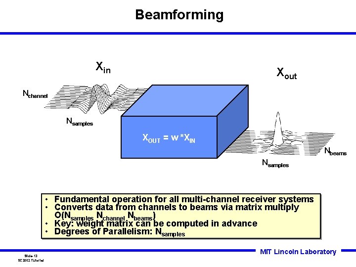
Beamforming Xin Xout Nchannel Nsamples XOUT = w *XIN Nbeams Nsamples • Fundamental operation for all multi-channel receiver systems • Converts data from channels to beams via matrix multiply O(Nsamples Nchannel Nbeams) • Key: weight matrix can be computed in advance • Degrees of Parallelism: Nsamples Slide-13 SC 2002 Tutorial MIT Lincoln Laboratory

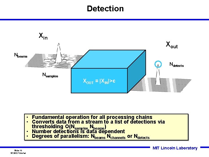
Detection Xin Xout Nbeams Ndetects Nsamples XOUT = |XIN|>c • Fundamental operation for all processing chains • Converts data from a stream to a list of detections via thresholding O(Nsamples Nbeams) • Number detections is data dependent • Degrees of parallelism: Nbeams Nchannels or Ndetects Slide-14 SC 2002 Tutorial MIT Lincoln Laboratory

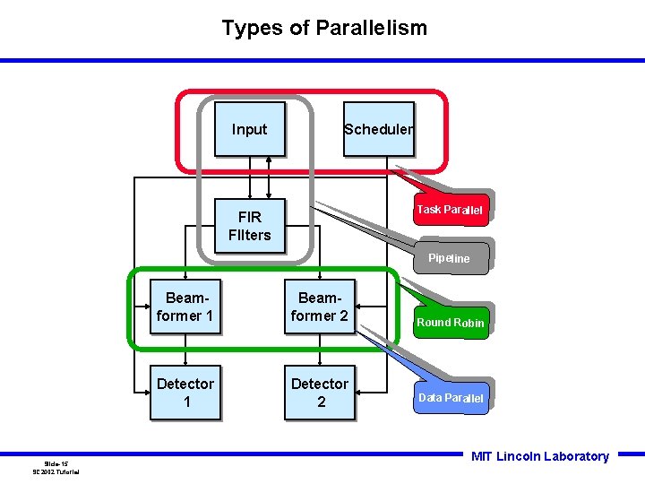
Types of Parallelism Input Scheduler Task Parallel FIR FIlters Pipeline Slide-15 SC 2002 Tutorial Beamformer 1 Beamformer 2 Detector 1 Detector 2 Round Robin Data Parallel MIT Lincoln Laboratory

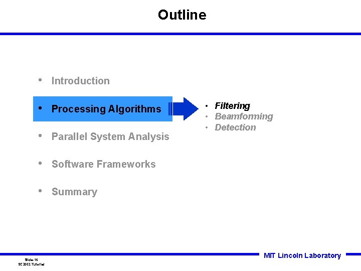
Outline • Introduction • Processing Algorithms • Parallel System Analysis • Software Frameworks • Summary Slide-16 SC 2002 Tutorial • Filtering • Beamforming • Detection MIT Lincoln Laboratory

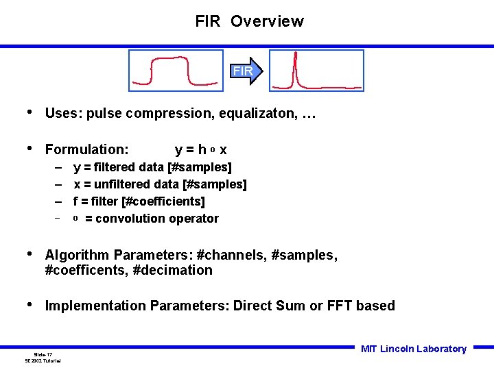
FIR Overview FIR • Uses: pulse compression, equalizaton, … • Formulation: y=hox – y = filtered data [#samples] – x = unfiltered data [#samples] – f = filter [#coefficients] – o = convolution operator • Algorithm Parameters: #channels, #samples, #coefficents, #decimation • Implementation Parameters: Direct Sum or FFT based Slide-17 SC 2002 Tutorial MIT Lincoln Laboratory

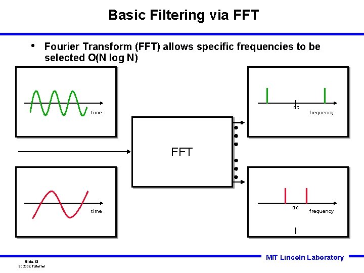
Basic Filtering via FFT • Fourier Transform (FFT) allows specific frequencies to be selected O(N log N) DC time frequency FFT time Slide-18 SC 2002 Tutorial DC frequency MIT Lincoln Laboratory

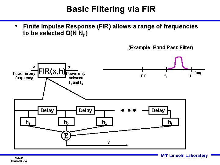
Basic Filtering via FIR • Finite Impulse Response (FIR) allows a range of frequencies to be selected O(N Nh) (Example: Band-Pass Filter) x Power in any frequency y FIR(x, h) Power only between f 1 and f 2 Delay h 1 DC Delay h 2 f 1 f 2 freq Delay h 3 h. L S y Slide-19 SC 2002 Tutorial MIT Lincoln Laboratory

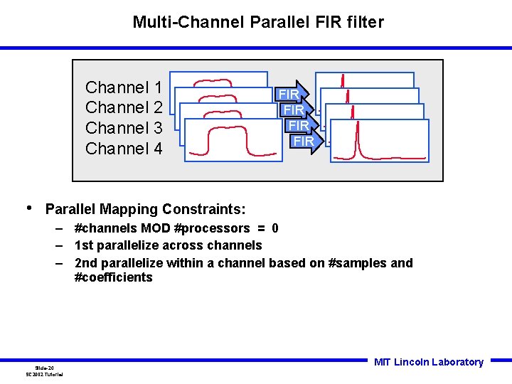
Multi-Channel Parallel FIR filter Channel 1 Channel 2 Channel 3 Channel 4 • FIR FIR Parallel Mapping Constraints: – #channels MOD #processors = 0 – 1 st parallelize across channels – 2 nd parallelize within a channel based on #samples and #coefficients Slide-20 SC 2002 Tutorial MIT Lincoln Laboratory

Outline • Introduction • Processing Algorithms • Parallel System Analysis • Software Frameworks • Summary Slide-21 SC 2002 Tutorial • Filtering • Beamforming • Detection MIT Lincoln Laboratory

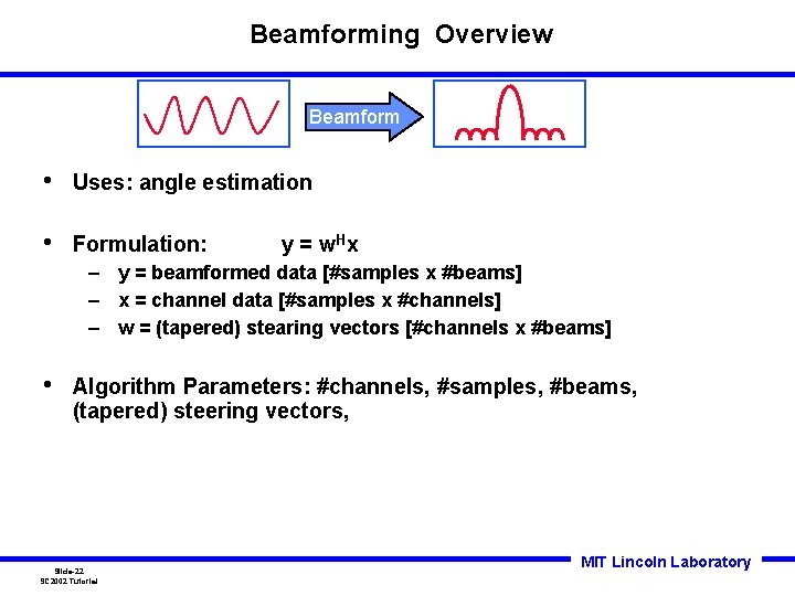
Beamforming Overview Beamform • Uses: angle estimation • Formulation: y = w. Hx – y = beamformed data [#samples x #beams] – x = channel data [#samples x #channels] – w = (tapered) stearing vectors [#channels x #beams] • Algorithm Parameters: #channels, #samples, #beams, (tapered) steering vectors, Slide-22 SC 2002 Tutorial MIT Lincoln Laboratory

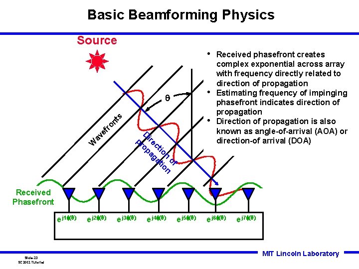
Basic Beamforming Physics Source • • W pr of n n io tio ct ga ire pa o D av ef ro nt s • Received phasefront creates complex exponential across array with frequency directly related to direction of propagation Estimating frequency of impinging phasefront indicates direction of propagation Direction of propagation is also known as angle-of-arrival (AOA) or direction-of arrival (DOA) Received Phasefront e j 1 Slide-23 SC 2002 Tutorial e j 2 e j 3 e j 4 e j 5 e j 6 e j 7 MIT Lincoln Laboratory

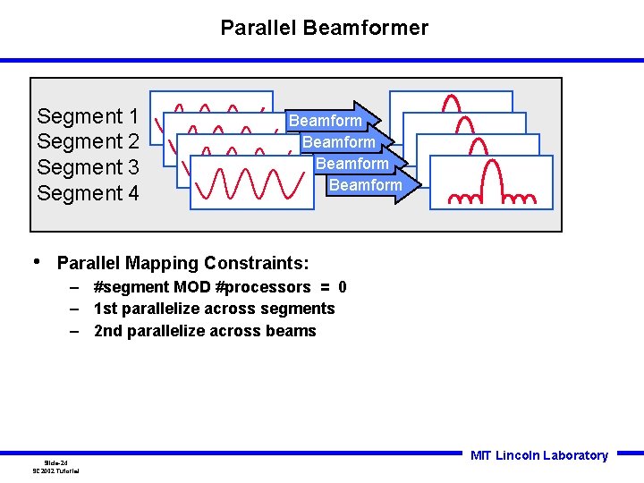
Parallel Beamformer Segment 1 Segment 2 Segment 3 Segment 4 • Beamform Parallel Mapping Constraints: – #segment MOD #processors = 0 – 1 st parallelize across segments – 2 nd parallelize across beams Slide-24 SC 2002 Tutorial MIT Lincoln Laboratory

Outline • Introduction • Processing Algorithms • Parallel System Analysis • Software Frameworks • Summary Slide-25 SC 2002 Tutorial • Filtering • Beamforming • Detection MIT Lincoln Laboratory

CFAR Detection Overview CFAR • Constant False Alarm Rate (CFAR) • Formulation: x[n] > T[n] – x[n] = cell under test – T[n] = Sum(xi)/2 M, Ngaurd < |i - N| < M + Ngaurd – Angle estimate: take ratio of beams; do lookup • Algorithm Parameters: #samples, #beams, steering vectors, #noise samples, #max detects • Implementation Parameters: Greatest Of, Censored Greatest Of, Ordered Statistics, … Averaging vs Sorting Slide-26 SC 2002 Tutorial MIT Lincoln Laboratory

Two-Pass Greatest-Of Excision CFAR (First Pass) Input Data x[i] M T T T T . . 1/M G G M L L L L . . 1/M Noise Estimate Buffer b[i] Range cell under test T Trailing training cells Guard cells L Leading training cells Reference: S. L. Wilson, Analysis of NRL’s two-pass greatest-of excision CFAR, Internal Memorandum, MIT Lincoln Laboratory, October 5 1998. Slide-27 SC 2002 Tutorial MIT Lincoln Laboratory

Two-Pass Greatest-Of Excision CFAR (Second Pass) Input Data x[i] Noise Estimate Buffer b[i] Slide-28 SC 2002 Tutorial T T T T M G G L L L L M Cell under test T Trailing training cells Guard cells L Leading training cells MIT Lincoln Laboratory

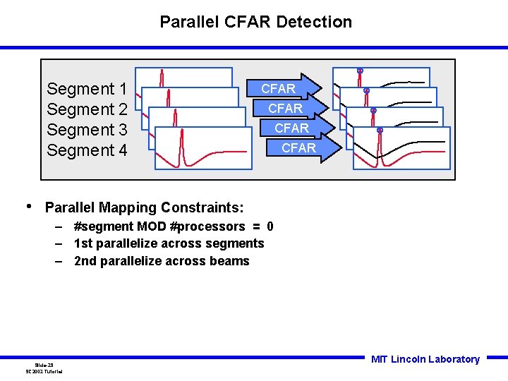
Parallel CFAR Detection Segment 1 Segment 2 Segment 3 Segment 4 • CFAR Parallel Mapping Constraints: – #segment MOD #processors = 0 – 1 st parallelize across segments – 2 nd parallelize across beams Slide-29 SC 2002 Tutorial MIT Lincoln Laboratory

Outline • Introduction • Processing Algorithms • Parallel System Analysis • Software Frameworks • Summary Slide-30 SC 2002 Tutorial • Latency vs. Throughput • Corner Turn • Dynamic Load Balancing MIT Lincoln Laboratory

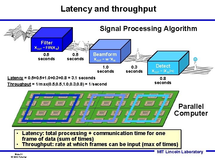
Latency and throughput Signal Processing Algorithm Filter XOUT = FIR(XIN) 0. 5 seconds Beamform XOUT = w *XIN 1. 0 seconds Latency = 0. 5+1. 0+0. 3+0. 8 = 3. 1 seconds Throughput = 1/max(0. 5, 1. 0, 0. 3, 0. 8) = 1/second 0. 3 seconds Detect XOUT = |XIN|>c 0. 8 seconds Parallel Computer • Latency: total processing + communication time for one frame of data (sum of times) • Throughput: rate at which frames can be input (max of times) Slide-31 SC 2002 Tutorial MIT Lincoln Laboratory

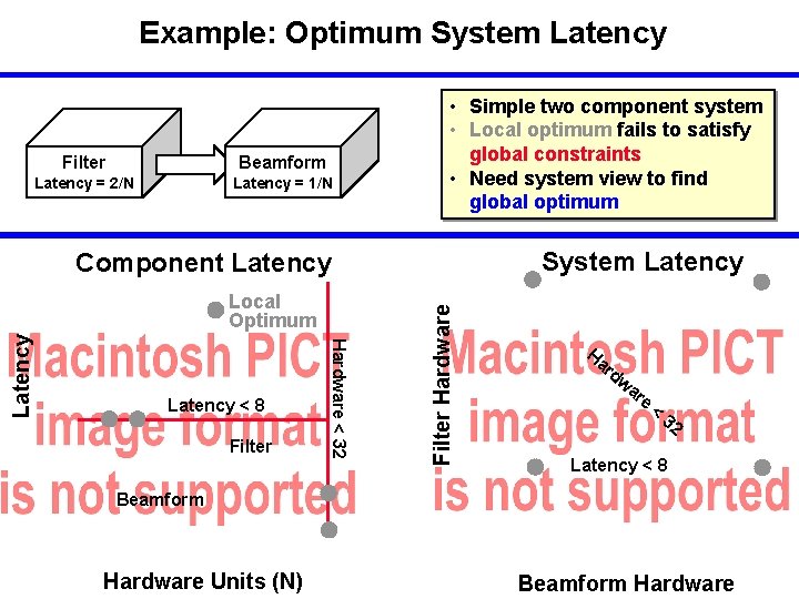
Example: Optimum System Latency Filter Beamform Latency = 2/N Latency = 1/N • Simple two component system • Local optimum fails to satisfy global constraints • Need system view to find global optimum System Latency < 8 Filter Hardware < 32 Latency Local Optimum Filter Hardware Component Latency Ha rd O Glo war pt b e im al < 32 um Latency < 8 Beamform Slide-32 SC 2002 Tutorial Hardware Units (N) MIT Lincoln Laboratory Beamform Hardware

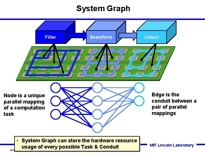
System Graph Filter Beamform Node is a unique parallel mapping of a computation task • System Graph can store the hardware resource usage of every possible Task & Conduit Slide-33 SC 2002 Tutorial Detect Edge is the conduit between a pair of parallel mappings MIT Lincoln Laboratory

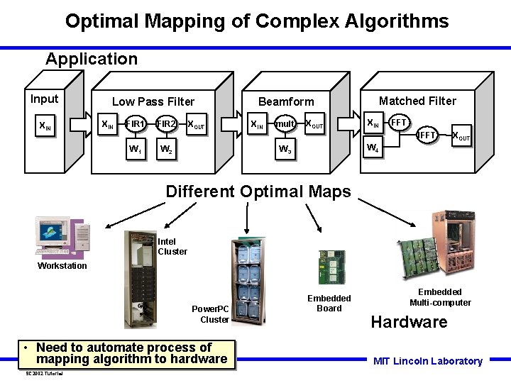
Optimal Mapping of Complex Algorithms Application Input XIN Low Pass Filter XIN FIR 1 W 1 FIR 2 XOUT XIN mult XOUT XIN FFT IFFT XOUT W 4 W 3 W 2 Matched Filter Beamform Different Optimal Maps Intel Cluster Workstation Power. PC Cluster • Need to automate process of mapping algorithm to hardware Slide-34 SC 2002 Tutorial Embedded Board Embedded Multi-computer Hardware MIT Lincoln Laboratory

Outline • Introduction • Processing Algorithms • Parallel System Analysis • Software Frameworks • Summary Slide-35 SC 2002 Tutorial • Latency vs. Throughput • Corner Turn • Dynamic Load Balancing MIT Lincoln Laboratory

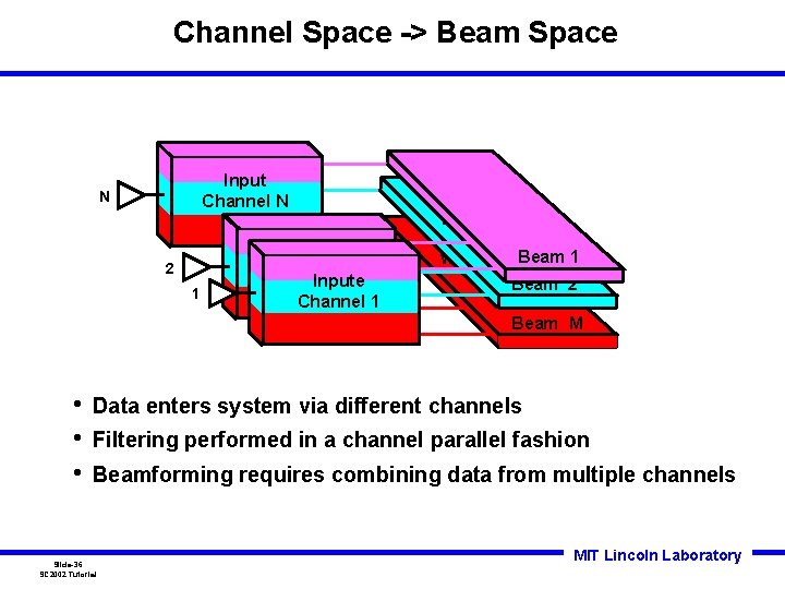
Channel Space -> Beam Space Input Channel N N 2 1 Weights Inpute Channel 1 Weights Beam 1 Beam 2 Beam M • • • Data enters system via different channels Filtering performed in a channel parallel fashion Beamforming requires combining data from multiple channels Slide-36 SC 2002 Tutorial MIT Lincoln Laboratory

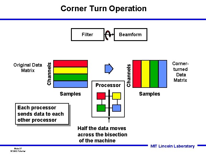
Corner Turn Operation Beamform Processor Cornerturned Data Matrix Channels Original Data Matrix Channels Filter Samples Each processor sends data to each other processor Half the data moves across the bisection of the machine Slide-37 SC 2002 Tutorial MIT Lincoln Laboratory

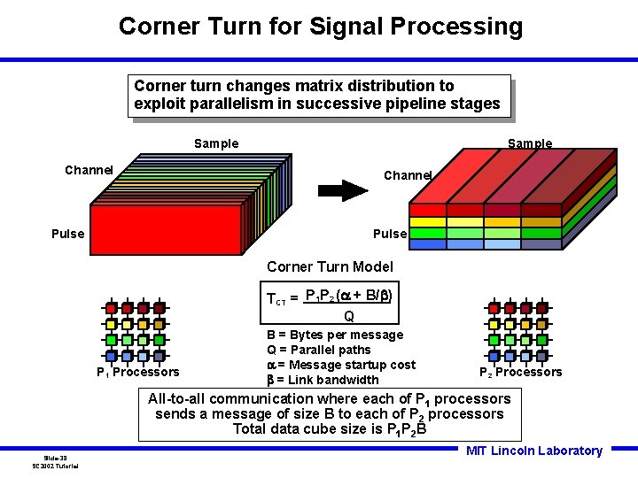
Corner Turn for Signal Processing Corner turn changes matrix distribution to exploit parallelism in successive pipeline stages Sample Channel Pulse Corner Turn Model TCT = P 1 P 2 ( + B/ ) Q P 1 Processors B = Bytes per message Q = Parallel paths = Message startup cost = Link bandwidth P 2 Processors All-to-all communication where each of P 1 processors sends a message of size B to each of P 2 processors Total data cube size is P 1 P 2 B Slide-38 SC 2002 Tutorial MIT Lincoln Laboratory

Outline • Introduction • Processing Algorithms • Parallel System Analysis • Software Frameworks • Summary Slide-39 SC 2002 Tutorial • Latency vs. Throughput • Corner Turn • Dynamic Load Balancing MIT Lincoln Laboratory

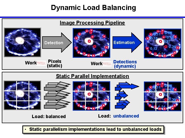
Dynamic Load Balancing Image Processing Pipeline Estimation Detection 0. 11 0. 15 0. 13 0. 08 0. 10 0. 97 0. 30 0. 24 Work Pixels (static) Work Detections (dynamic) Static Parallel Implementation 0. 11 0. 15 0. 13 0. 08 0. 10 0. 97 0. 30 0. 24 Load: balanced Slide-40 SC 2002 Tutorial Load: unbalanced • Static parallelism implementations lead to unbalanced loads MIT Lincoln Laboratory

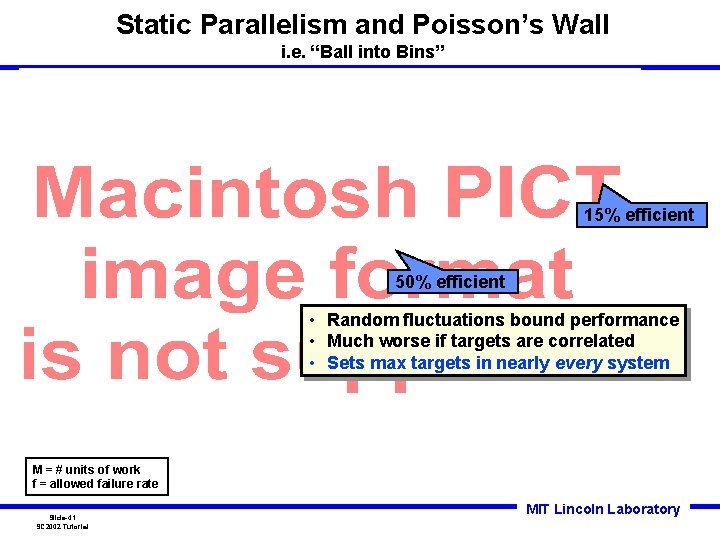
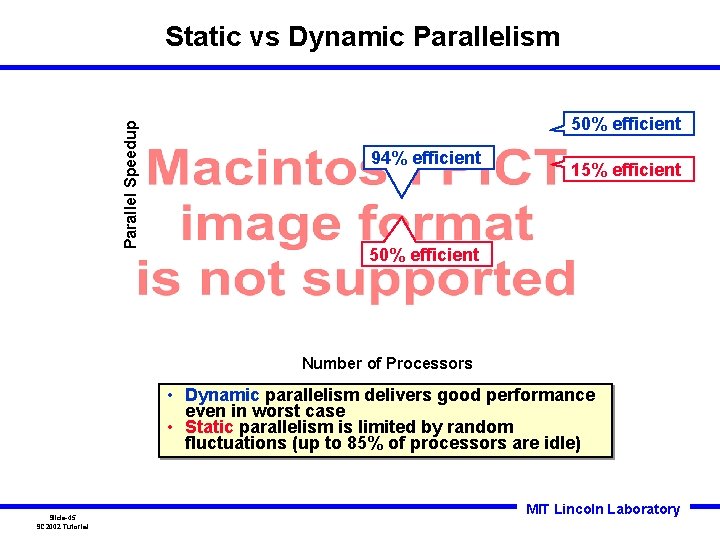
Static Parallelism and Poisson’s Wall i. e. “Ball into Bins” 15% efficient 50% efficient • Random fluctuations bound performance • Much worse if targets are correlated • Sets max targets in nearly every system M = # units of work f = allowed failure rate Slide-41 SC 2002 Tutorial MIT Lincoln Laboratory

Static Derivation Slide-42 SC 2002 Tutorial MIT Lincoln Laboratory

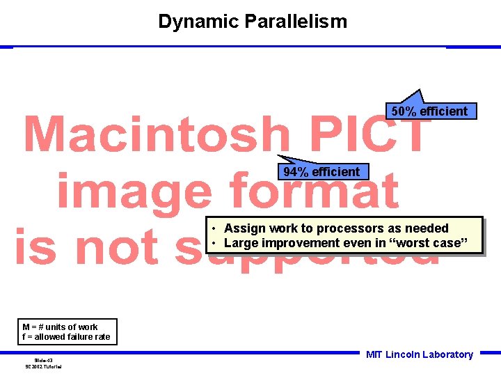
Dynamic Parallelism 50% efficient 94% efficient • Assign work to processors as needed • Large improvement even in “worst case” M = # units of work f = allowed failure rate Slide-43 SC 2002 Tutorial MIT Lincoln Laboratory

Dynamic Derivation Slide-44 SC 2002 Tutorial MIT Lincoln Laboratory

Parallel Speedup Static vs Dynamic Parallelism 50% efficient 94% efficient 15% efficient 50% efficient Number of Processors • Dynamic parallelism delivers good performance even in worst case • Static parallelism is limited by random fluctuations (up to 85% of processors are idle) Slide-45 SC 2002 Tutorial MIT Lincoln Laboratory

Outline • Introduction • Processing Algorithms • Parallel System Analysis • Software Frameworks • Summary Slide-46 SC 2002 Tutorial • • PVL PETE S 3 P Matlab. MPI MIT Lincoln Laboratory

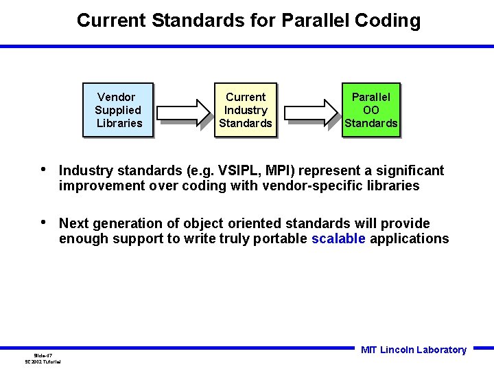
Current Standards for Parallel Coding Vendor Supplied Libraries Current Industry Standards Parallel OO Standards • Industry standards (e. g. VSIPL, MPI) represent a significant improvement over coding with vendor-specific libraries • Next generation of object oriented standards will provide enough support to write truly portable scalable applications Slide-47 SC 2002 Tutorial MIT Lincoln Laboratory

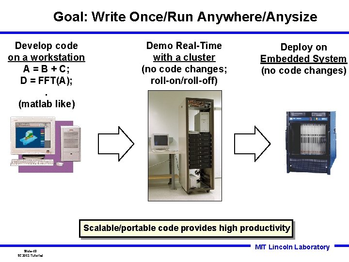
Goal: Write Once/Run Anywhere/Anysize Develop code on a workstation A = B + C; D = FFT(A); . (matlab like) Demo Real-Time with a cluster (no code changes; roll-on/roll-off) Deploy on Embedded System (no code changes) Scalable/portable code provides high productivity Slide-48 SC 2002 Tutorial MIT Lincoln Laboratory

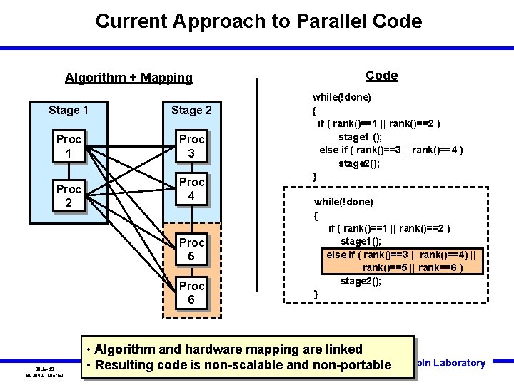
Current Approach to Parallel Code Algorithm + Mapping Stage 1 Stage 2 Proc 1 Proc 3 Proc 2 Proc 4 Proc 5 Proc 6 Slide-49 SC 2002 Tutorial Code while(!done) { if ( rank()==1 || rank()==2 ) stage 1 (); else if ( rank()==3 || rank()==4 ) stage 2(); } while(!done) { if ( rank()==1 || rank()==2 ) stage 1(); else if ( rank()==3 || rank()==4) || rank()==5 || rank==6 ) stage 2(); } • Algorithm and hardware mapping are linked MIT Lincoln Laboratory • Resulting code is non-scalable and non-portable

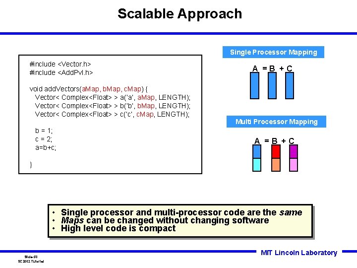
Scalable Approach Single Processor Mapping #include <Vector. h> #include <Add. Pvl. h> A =B +C void add. Vectors(a. Map, b. Map, c. Map) { Vector< Complex<Float> > a(‘a’, a. Map, LENGTH); Vector< Complex<Float> > b(‘b’, b. Map, LENGTH); Vector< Complex<Float> > c(‘c’, c. Map, LENGTH); Multi Processor Mapping b = 1; c = 2; a=b+c; A =B +C } • Single processor and multi-processor code are the same • Maps can be changed without changing software • High level code is compact Slide-50 SC 2002 Tutorial MIT Lincoln Laboratory

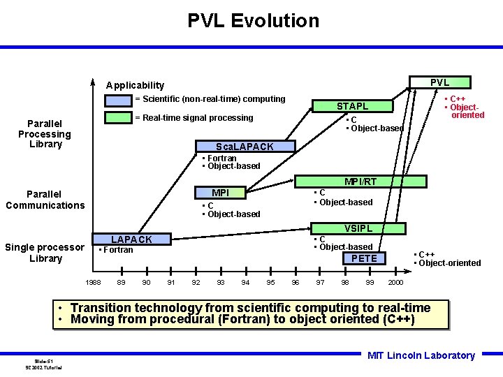
PVL Evolution PVL Applicability = Scientific (non-real-time) computing = Real-time signal processing Parallel Processing Library • C++ • Objectoriented STAPL • C • Object-based Sca. LAPACK • Fortran • Object-based MPI/RT MPI Parallel Communications Single processor Library • C • Object-based VSIPL LAPACK • C • Object-based • Fortran 1988 89 • C++ • Object-oriented PETE 90 91 92 93 94 95 96 97 98 99 2000 • Transition technology from scientific computing to real-time • Moving from procedural (Fortran) to object oriented (C++) Slide-51 SC 2002 Tutorial MIT Lincoln Laboratory

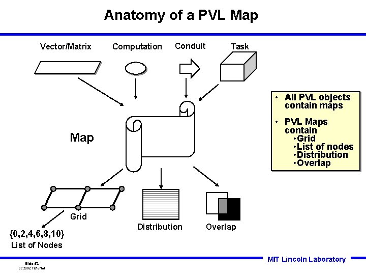
Anatomy of a PVL Map Vector/Matrix Computation Conduit Task • All PVL objects contain maps • PVL Maps contain • Grid • List of nodes • Distribution • Overlap Map Grid {0, 2, 4, 6, 8, 10} Distribution Overlap List of Nodes Slide-52 SC 2002 Tutorial MIT Lincoln Laboratory

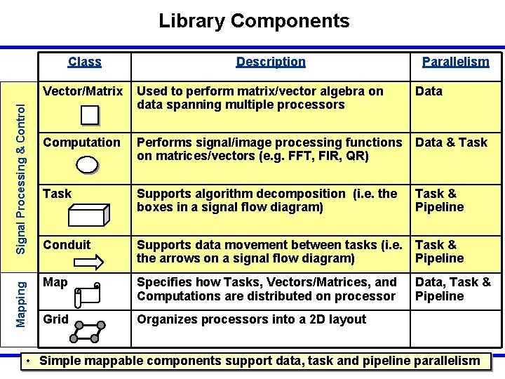
Library Components Mapping Signal Processing & Control Class Description Parallelism Vector/Matrix Used to perform matrix/vector algebra on data spanning multiple processors Data Computation Performs signal/image processing functions Data & Task on matrices/vectors (e. g. FFT, FIR, QR) Task Supports algorithm decomposition (i. e. the boxes in a signal flow diagram) Conduit Supports data movement between tasks (i. e. Task & the arrows on a signal flow diagram) Pipeline Map Specifies how Tasks, Vectors/Matrices, and Computations are distributed on processor Grid Organizes processors into a 2 D layout Task & Pipeline Data, Task & Pipeline MIT Lincoln Laboratory • Simple mappable components support data, task and pipeline parallelism Slide-53 SC 2002 Tutorial

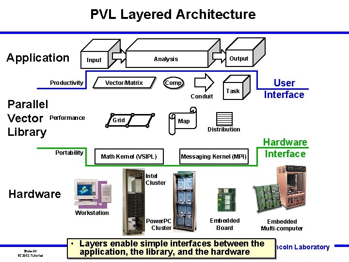
PVL Layered Architecture Application Productivity Vector/Matrix Comp Conduit Parallel Vector Performance Library Portability Output Analysis Input Grid Task User Interface Map Distribution Math Kernel (VSIPL) Messaging Kernel (MPI) Hardware Interface Intel Cluster Hardware Workstation Power. PC Cluster Slide-54 SC 2002 Tutorial Embedded Board Embedded Multi-computer • Layers enable simple interfaces between the MIT Lincoln Laboratory application, the library, and the hardware

Outline • Introduction • Processing Algorithms • Parallel System Analysis • Software Frameworks • Summary Slide-55 SC 2002 Tutorial • • PVL PETE S 3 P Matlab. MPI MIT Lincoln Laboratory

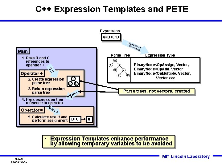
C++ Expression Templates and PETE Expression A=B+C*D Exp res Tem plasion tes Main Parse Tree 1. Pass B and C references to operator + Operator + Binary. Node<Op. Assign, Vector, Binary. Node<Op. Add, Vector Binary. Node<Op. Multiply, Vector >>> , B& & C 2. Create expression parse tree 3. Return expression parse tree + B& Expression Type C& Parse trees, not vectors, created py co 4. Pass expression tree reference to operator Operator = co py & 5. Calculate result and perform assignment B+C A • Expression Templates enhance performance by allowing temporary variables to be avoided Slide-56 SC 2002 Tutorial MIT Lincoln Laboratory

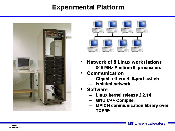
Experimental Platform Slide-57 SC 2002 Tutorial • Network of 8 Linux workstations • Communication • Software – 800 MHz Pentium III processors – Gigabit ethernet, 8 -port switch – Isolated network – Linux kernel release 2. 2. 14 – GNU C++ Compiler – MPICH communication library over TCP/IP MIT Lincoln Laboratory

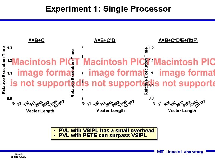
Experiment 1: Single Processor A=B+C*D 1. 2 1. 1 1 0. 9 2 8 32 128 512 048 192 2768 107 2 8 3 13 Vector Length 1. 2 1. 1 1 0. 9 0. 8 0. 7 0. 6 A=B+C*D/E+fft(F) Relative Execution Time 1. 3 Relative Execution Time A=B+C 2 8 32 128 512 048 192 2768 107 2 8 3 13 Vector Length 1. 2 1. 1 1 0. 9 0. 8 2 8 32 128 512 048 192 2768 107 2 8 3 13 Vector Length • PVL with VSIPL has a small overhead • PVL with PETE can surpass VSIPL Slide-58 SC 2002 Tutorial MIT Lincoln Laboratory

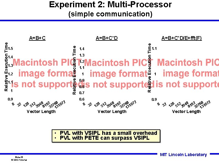
Experiment 2: Multi-Processor (simple communication) 1. 5 1. 4 1. 3 1. 2 1. 1 1 0. 9 2 8 32 128 512 048 192 2768 107 2 8 3 13 Vector Length A=B+C*D/E+fft(F) Relative Execution Time A=B+C*D Relative Execution Time A=B+C 1. 1 1. 4 1. 3 1. 2 1. 1 1 0. 9 0. 8 0. 7 0. 6 2 8 32 128 512 048 192 2768 107 2 8 3 13 1 0. 9 Vector Length 2 8 32 128 512 048 192 2768 107 2 8 3 13 Vector Length • PVL with VSIPL has a small overhead • PVL with PETE can surpass VSIPL Slide-59 SC 2002 Tutorial MIT Lincoln Laboratory

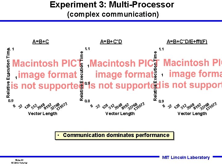
Experiment 3: Multi-Processor (complex communication) A=B+C*D 1. 1 1 0. 9 2 8 32 128 512 048 192 2768 107 2 8 3 13 Vector Length 1. 1 Relative Execution Time 1. 1 1 A=B+C*D/E+fft(F) 1 0. 9 0. 8 2 8 32 128 512 048 192 2768 107 2 8 3 13 Vector Length 1 0. 9 2 8 32 128 512 048 192 2768 107 2 8 3 13 Vector Length • Communication dominates performance Slide-60 SC 2002 Tutorial MIT Lincoln Laboratory

Outline • Introduction • Processing Algorithms • Parallel System Analysis • Software Frameworks • Summary Slide-61 SC 2002 Tutorial • • PVL PETE S 3 P Matlab. MPI MIT Lincoln Laboratory

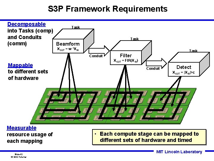
S 3 P Framework Requirements Decomposable Task into Tasks (comp) and Conduits (comm) Beamform Task XOUT = w *XIN Task Conduit Mappable to different sets of hardware Measurable resource usage of each mapping Slide-62 SC 2002 Tutorial Filter XOUT = FIR(XIN) Conduit Detect XOUT = |XIN|>c • Each compute stage can be mapped to different sets of hardware and timed MIT Lincoln Laboratory

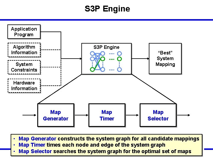
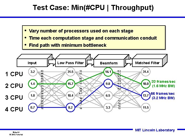
S 3 P Engine Application Program Algorithm Information S 3 P Engine “Best” System Mapping System Constraints Hardware Information Map Generator Map Timer Map Selector • Map Generator constructs the system graph for all candidate mappings • Map Timer times each node and edge of the system graph MITset Lincoln Laboratory • Map Selector searches the system graph for the optimal of maps Slide-63 SC 2002 Tutorial

Test Case: Min(#CPU | Throughput) • • • Vary number of processors used on each stage Time each computation stage and communication conduit Find path with minimum bottleneck Input 1 CPU 3. 2 2 CPU 1. 4 3 CPU 1. 0 4 CPU 0. 7 Slide-64 SC 2002 Tutorial Low Pass Filter 52 49 46 42 47 27 21 24 44 29 20 24 60 33 23 15 31. 5 15. 7 10. 4 8. 2 12 31 57 16 17 28 14 9. 1 18 18 15 14 Beamform 16. 1 9. 8 6. 5 3. 3 8. 7 3. 3 2. 6 7. 3 8. 3 9. 4 8. 0 17 14 14 13 Matched Filter 31. 4 18. 0 33 frames/sec (1. 6 MHz BW) 13. 7 66 frames/sec (3. 2 MHz BW) 11. 5 MIT Lincoln Laboratory

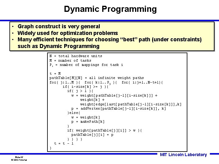
Dynamic Programming • Graph construct is very general • Widely used for optimization problems • Many efficient techniques for choosing “best” path (under constraints) such as Dynamic Programming N = total hardware units M = number of tasks Pi = number of mappings for task i t = M path. Table[M][N] = all infinite weight paths for( j: 1. . M ){ for( k: 1. . Pj ){ for( i: j+1. . N-t+1){ if( i-size[k] >= j ){ if( j > 1 ){ w = weight[path. Table[j-1][i-size[k]]] + weight[k] + weight[edge[last[ path. Table[j-1][i-size[k]]], k] p = add. Vertex[path. Table[j-1][i-size[k]], k] }else{ w = weight[k] p = make. Path[k] } if( weight[path. Table[j][i]] > w ){ path. Table[j][i] = p } } t = t - 1 } Slide-65 SC 2002 Tutorial MIT Lincoln Laboratory

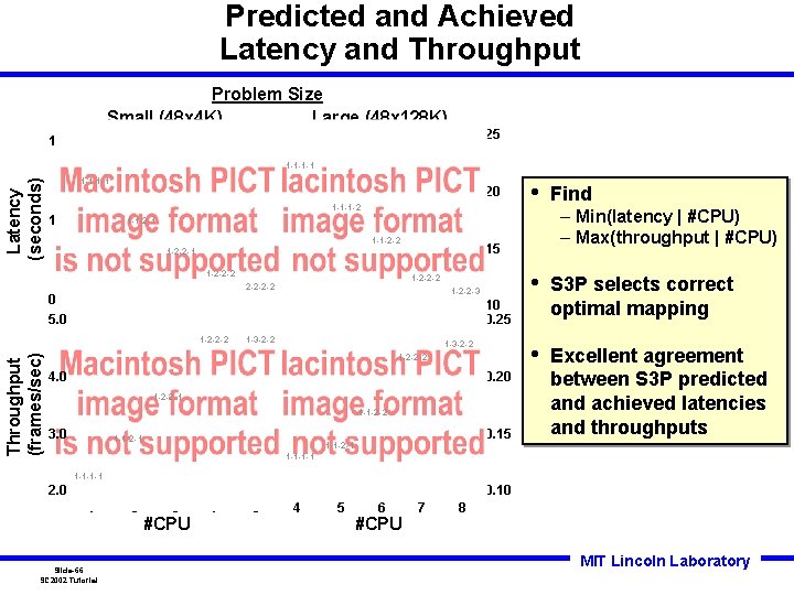
Predicted and Achieved Latency and Throughput Problem Size Small (48 x 4 K) Large (48 x 128 K) 25 1. 5 Latency (seconds) 1 -1 -1 -1 20 1 -1 -1 -2 1. 0 Find • S 3 P selects correct optimal mapping • Excellent agreement between S 3 P predicted and achieved latencies and throughputs 1 -1 -2 -1 1 -1 -2 -2 15 1 -2 -2 -1 1 -2 -2 -2 -2 0. 5 5. 0 1 -2 -2 -3 10 0. 25 1 -2 -2 -2 Throughput (frames/sec) • 1 -3 -2 -2 1 -2 -2 -2 4. 0 0. 20 1 -2 -2 -1 1 -1 -2 -2 3. 0 0. 15 1 -1 -2 -1 – Min(latency | #CPU) – Max(throughput | #CPU) 1 -1 -2 -1 1 -1 -1 -1 2. 0 0. 10 4 Slide-66 SC 2002 Tutorial 5 6 #CPU 7 8 4 5 6 #CPU 7 8 MIT Lincoln Laboratory

Outline • Introduction • Processing Algorithms • Parallel System Analysis • Software Frameworks • Summary Slide-67 SC 2002 Tutorial • • PVL PETE S 3 P Matlab. MPI MIT Lincoln Laboratory

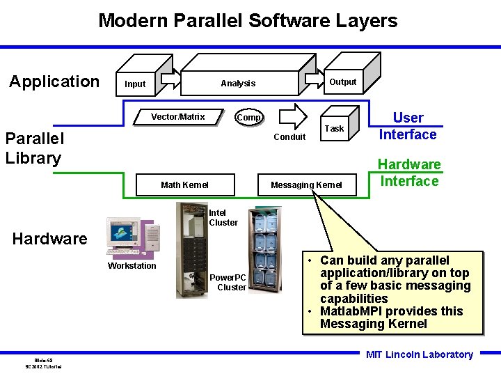
Modern Parallel Software Layers Application Output Analysis Input Vector/Matrix Comp Parallel Library Conduit Task Messaging Kernel Math Kernel User Interface Hardware Interface Intel Cluster Hardware Workstation Power. PC Cluster Slide-68 SC 2002 Tutorial • Can build any parallel application/library on top of a few basic messaging capabilities • Matlab. MPI provides this Messaging Kernel MIT Lincoln Laboratory

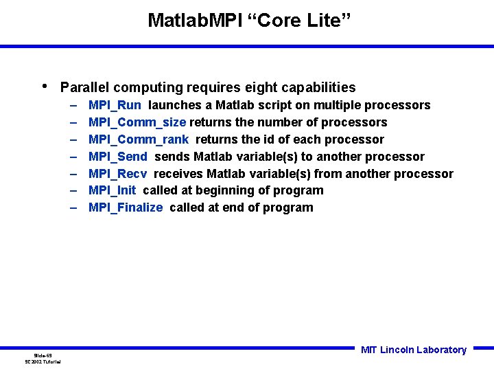
Matlab. MPI “Core Lite” • Parallel computing requires eight capabilities – – – – Slide-69 SC 2002 Tutorial MPI_Run launches a Matlab script on multiple processors MPI_Comm_size returns the number of processors MPI_Comm_rank returns the id of each processor MPI_Send sends Matlab variable(s) to another processor MPI_Recv receives Matlab variable(s) from another processor MPI_Init called at beginning of program MPI_Finalize called at end of program MIT Lincoln Laboratory

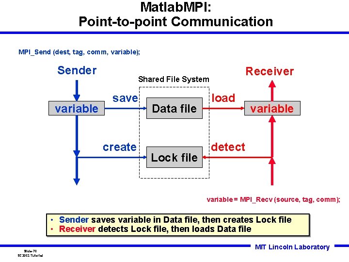
Matlab. MPI: Point-to-point Communication MPI_Send (dest, tag, comm, variable); Sender variable Receiver Shared File System save create Data file Lock file load variable detect variable = MPI_Recv (source, tag, comm); • Sender saves variable in Data file, then creates Lock file • Receiver detects Lock file, then loads Data file Slide-70 SC 2002 Tutorial MIT Lincoln Laboratory

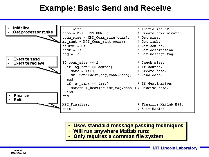
Example: Basic Send and Receive • Initialize • Get processor ranks • Execute send • Execute recieve • Finalize • Exit MPI_Init; comm = MPI_COMM_WORLD; comm_size = MPI_Comm_size(comm); my_rank = MPI_Comm_rank(comm); source = 0; dest = 1; tag = 1; % % % % Initialize MPI. Create communicator. Get size. Get rank. Set source. Set destination. Set message tag. if(comm_size == 2) if (my_rank == source) data = 1: 10; MPI_Send(dest, tag, comm, data); end if (my_rank == dest) data=MPI_Recv(source, tag, comm); end % % Check size. If source. Create data. Send data. MPI_Finalize; exit; % Finalize Matlab MPI. % Exit Matlab % If destination. % Receive data. • Uses standard message passing techniques • Will run anywhere Matlab runs • Only requires a common file system Slide-71 SC 2002 Tutorial MIT Lincoln Laboratory

Matlab. MPI vs MPI bandwidth Bandwidth (Bytes/sec) Bandwidth (SGI Origin 2000) Message Size (Bytes) • Bandwidth matches native C MPI at large message size • Primary difference is latency (35 milliseconds vs. 30 MIT microseconds) Lincoln Laboratory Slide-72 SC 2002 Tutorial

Image Filtering Parallel Performance Scaled Problem Size (IBM SP 2) Gigaflops Speedup Fixed Problem (SGI O 2000) Parallel. Size performance Number of Processors • Achieved “classic” super-linear speedup on fixed problem • Achieved speedup of ~300 on 304 processors on scaled problem Slide-73 SC 2002 Tutorial MIT Lincoln Laboratory

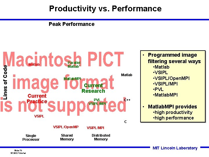
Productivity vs. Performance Peak Performance Lines of Code Matlab • Programmed image filtering several ways Parallel Matlab* Matlab. MPI Current Research Current Practice PVL VSIPL/MPI C++ • Matlab. MPI provides VSIPL C VSIPL/Open. MP Single Processor Slide-74 SC 2002 Tutorial Shared Memory • Matlab • VSIPL/Open. MPI • VSIPL/MPI • PVL • Matlab. MPI • high productivity • high performance VSIPL/MPI Distributed Memory MIT Lincoln Laboratory

Summary • Exploiting parallel processing for streaming applications presents unique software challenges. • The community is developing software librariea to address many of these challenges: – – • Exploits C++ to easily express data/task parallelism Seperates parallel hardware dependencies from software Allows a variety of strategies for implementing dynamic applications(e. g. for fault tolerance) Delivers high performance execution comparable to or better than standard approaches Our future efforts will focus on adding to and exploiting the features of this technology to: – – – Slide-75 SC 2002 Tutorial Exploit dynamic parallelism Integrate high performance parallel software underneath mainstream programming environments (e. g Matlab, IDL, …) Use self-optimizing techniques to maintain performance MIT Lincoln Laboratory