DNN Accelerator Architectures Thanks to Joel Emer Vivienne

DNN Accelerator Architectures Thanks to Joel Emer, Vivienne Sze, Yu-Hsin Chen 1

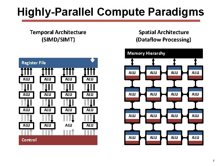
Highly-Parallel Compute Paradigms Temporal Architecture (SIMD/SIMT) Spatial Architecture (Dataflow Processing) Memory Hierarchy Register File ALU ALU ALU ALU Control ALU ALU ALU ALU ALU 2

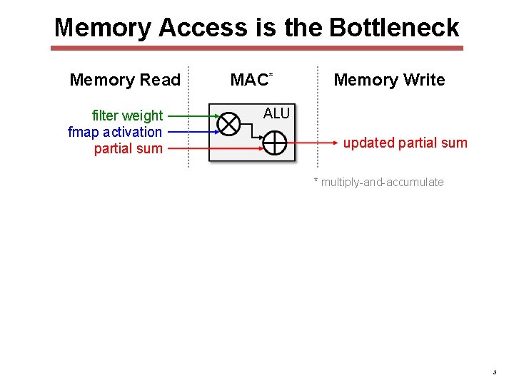
Memory Access is the Bottleneck Memory Read filter weight fmap activation partial sum MAC* Memory Write ALU updated partial sum * multiply-and-accumulate 3

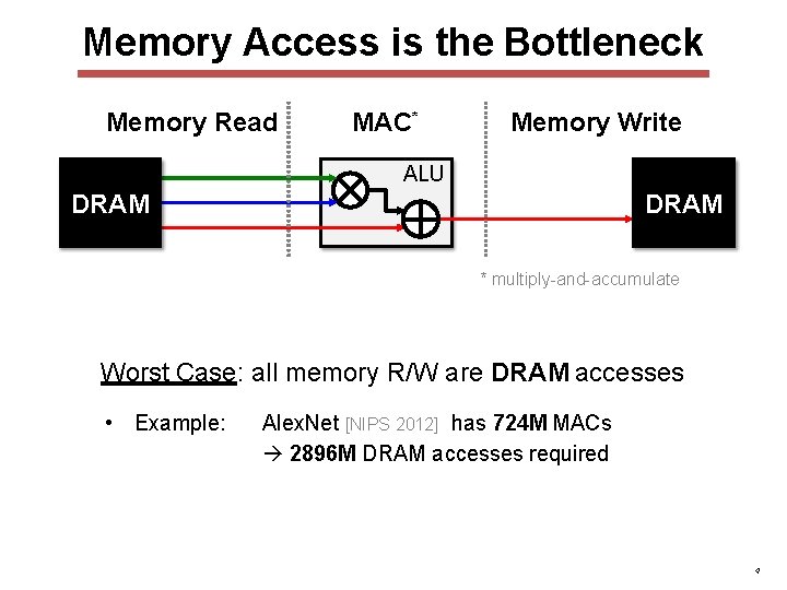
Memory Access is the Bottleneck Memory Read MAC* Memory Write ALU DRAM * multiply-and-accumulate Worst Case: all memory R/W are DRAM accesses • Example: Alex. Net [NIPS 2012] has 724 M MACs 2896 M DRAM accesses required 4

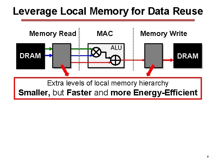
Leverage Local Memory for Data Reuse Memory Read MAC Memory Write ALU DRAM Extra levels of local memory hierarchy Smaller, but Faster and more Energy-Efficient 5

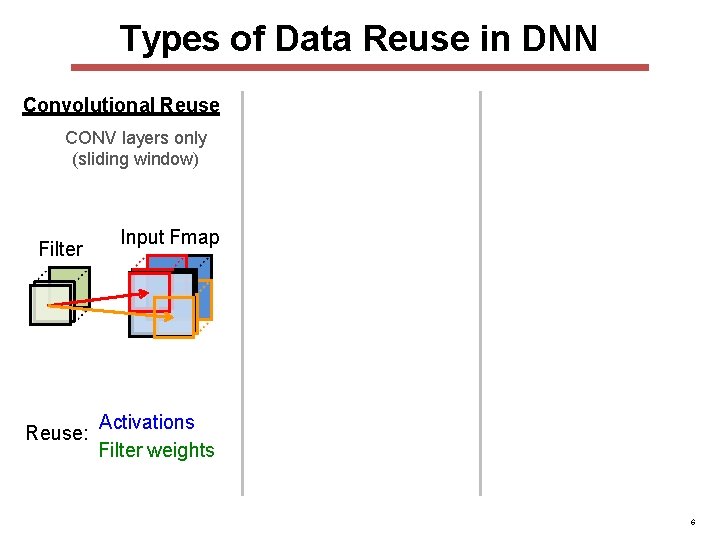
Types of Data Reuse in DNN Convolutional Reuse CONV layers only (sliding window) Filter Reuse: Input Fmap Activations Filter weights 6

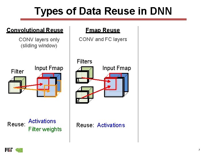
Types of Data Reuse in DNN Convolutional Reuse CONV layers only (sliding window) Fmap Reuse CONV and FC layers Filter Input Fmap 1 2 Reuse: Activations Filter weights Reuse: Activations 7

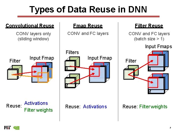
Types of Data Reuse in DNN Convolutional Reuse CONV layers only (sliding window) Fmap Reuse Filter Reuse CONV and FC layers (batch size > 1) Input Fmaps Filter Input Fmap 1 Filter 1 2 2 Reuse: Activations Filter weights Reuse: Activations Reuse: Filter weights 8

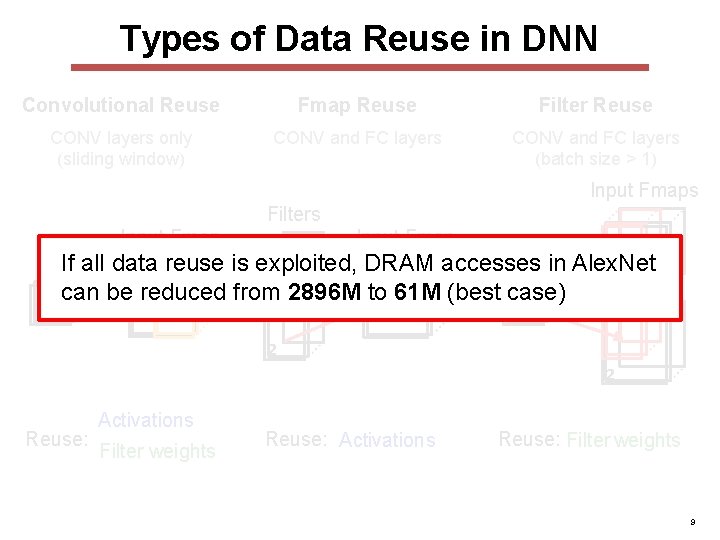
Types of Data Reuse in DNN Convolutional Reuse Fmap Reuse Filter Reuse CONV layers only (sliding window) CONV and FC layers (batch size > 1) Input Fmaps Filter Input Fmap Filter If all data reuse is exploited, DRAM accesses in Alex. Net 1 1 can be reduced from 2896 M to 61 M (best case) 2 2 Reuse: Activations Filter weights Reuse: Activations Reuse: Filter weights 9

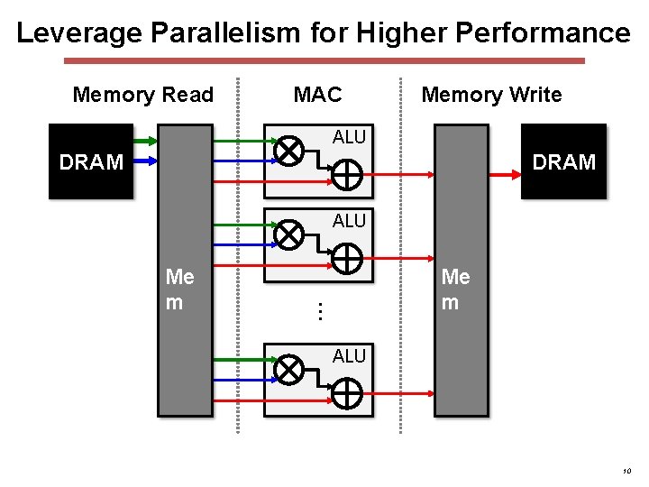
Leverage Parallelism for Higher Performance Memory Read MAC Memory Write ALU DRAM ALU … Me m ALU 10

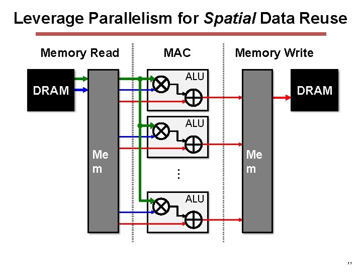
Leverage Parallelism for Spatial Data Reuse Memory Read MAC Memory Write ALU DRAM ALU … Me m ALU 11

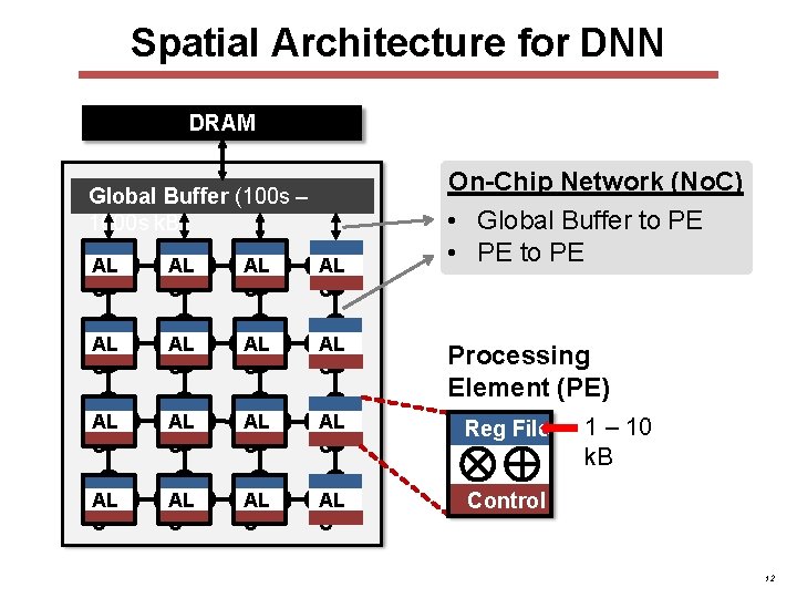
Spatial Architecture for DNN DRAM Global Buffer (100 s – 1000 s k. B) On-Chip Network (No. C) • Global Buffer to PE • PE to PE AL U AL U AL U Reg File AL U Control Processing Element (PE) 1 – 10 k. B 12

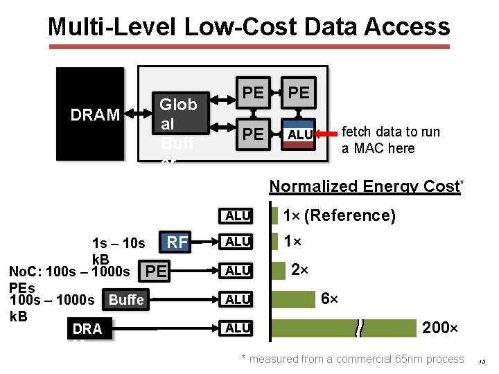
Multi-Level Low-Cost Data Access DRAM Glob al Buff er PE PE PE ALU fetch data to run a MAC here Normalized Energy Cost* 1 s – 10 s RF k. B No. C: 100 s – 1000 s PE PEs 100 s – 1000 s Buffe k. B r DRA M ALU 1× (Reference) ALU 1× ALU ALU 2× 6× 200× * measured from a commercial 65 nm process 13

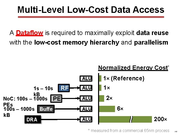
Multi-Level Low-Cost Data Access A Dataflow is required to maximally exploit data reuse with the low-cost memory hierarchy and parallelism Normalized Energy Cost* 1 s – 10 s RF k. B No. C: 100 s – 1000 s PE PEs 100 s – 1000 s Buffe k. B r DRA M ALU 1× (Reference) ALU 1× ALU ALU 2× 6× 200× * measured from a commercial 65 nm process 14

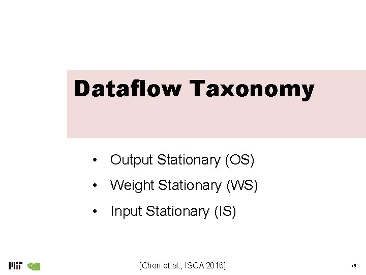
Dataflow Taxonomy • Output Stationary (OS) • Weight Stationary (WS) • Input Stationary (IS) [Chen et al. , ISCA 2016] 15

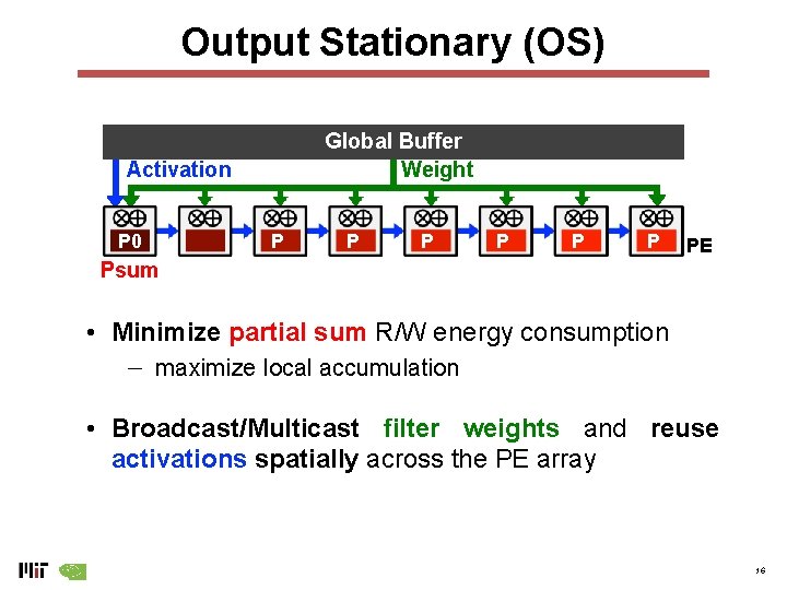
Output Stationary (OS) Global Buffer Weight Activation P 0 Psum P 1 P 2 P 3 P 4 P 5 P 6 P 7 PE • Minimize partial sum R/W energy consumption − maximize local accumulation • Broadcast/Multicast filter weights and reuse activations spatially across the PE array 16

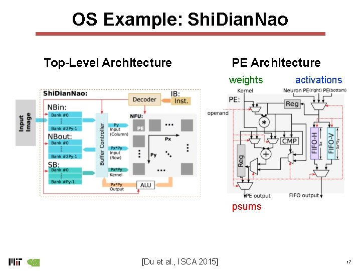
OS Example: Shi. Dian. Nao Top-Level Architecture PE Architecture weights activations psums [Du et al. , ISCA 2015] 17

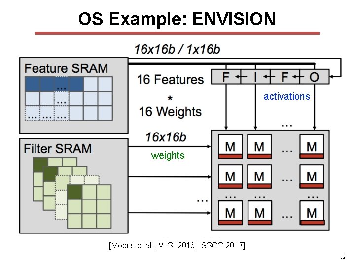
OS Example: ENVISION activations weights [Moons et al. , VLSI 2016, ISSCC 2017] 18

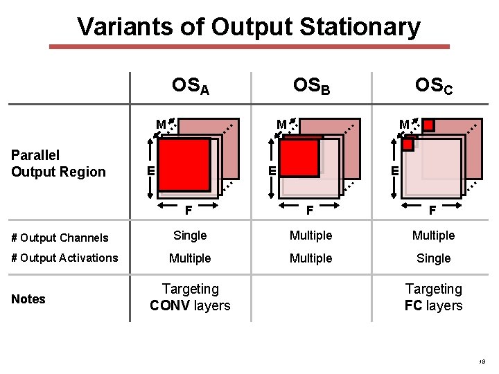
Variants of Output Stationary # Output Channels # Output Activations Notes M … … E E … … E OSC … … Parallel Output Region M … … M OSB … OSA F F F Single Multiple Single Targeting CONV layers Targeting FC layers 19

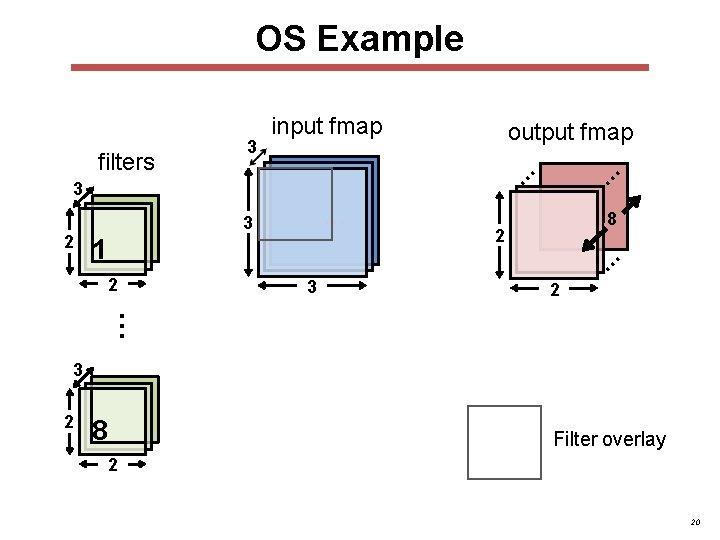
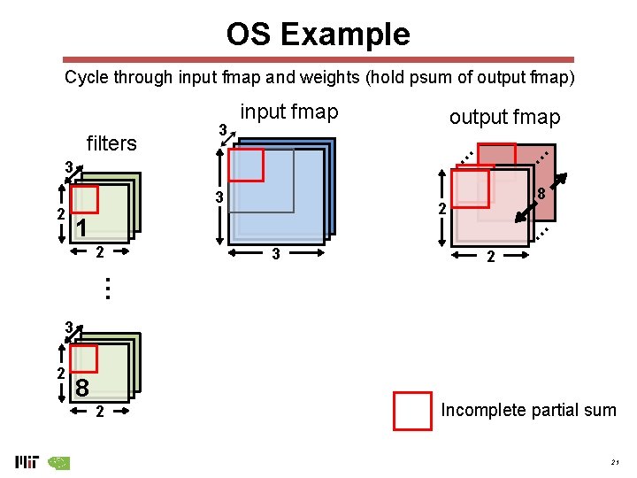
OS Example output fmap 3 1 8 2 … 3 … … filters 3 input fmap 3 2 … 2 3 2 8 Filter overlay 2 20

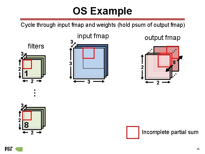
OS Example Cycle through input fmap and weights (hold psum of output fmap) output fmap 3 8 2 1 … 2 3 … … filters 3 input fmap 3 2 … 2 3 2 8 2 Incomplete partial sum 21

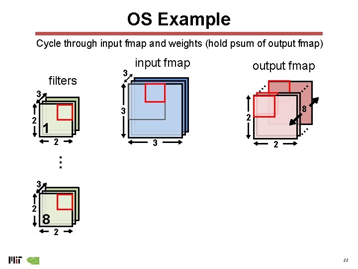
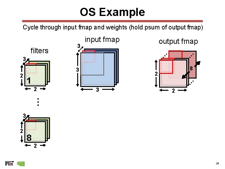
OS Example Cycle through input fmap and weights (hold psum of output fmap) output fmap 3 8 2 1 … 2 3 … … filters 3 input fmap 3 2 … 2 3 2 8 2 22

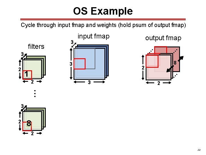
OS Example Cycle through input fmap and weights (hold psum of output fmap) output fmap 3 8 2 1 … 2 3 … … filters 3 input fmap 3 2 … 2 3 2 88 2 23

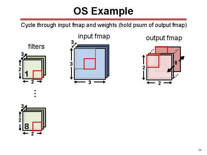
OS Example Cycle through input fmap and weights (hold psum of output fmap) output fmap 3 8 2 1 … 2 3 … … filters 3 input fmap 3 2 … 2 3 2 8 2 24

OS Example Cycle through input fmap and weights (hold psum of output fmap) output fmap 3 8 2 1 … 2 3 … … filters 3 input fmap 3 2 … 2 3 2 8 2 25

OS Example Cycle through input fmap and weights (hold psum of output fmap) output fmap 3 8 2 1 … 2 3 … … filters 3 input fmap 3 2 … 2 3 2 8 2 Incomplete partial sum 26

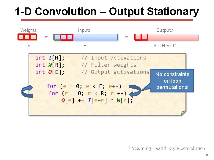
1 -D Convolution – Output Stationary Weights Inputs = * R Outputs H int I[H]; int W[R]; int O[E]; E = H-R+1† // Input activations // Filter weights // Output activations for (e = 0; e < E; e++) for (r = 0; r < R; r ++) O[e] += I[e+r] * W[r]; † Assuming: No constraints on loop permutations! ‘valid’ style convolution 27

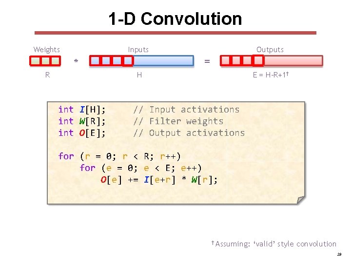
1 -D Convolution Weights Inputs = * R Outputs H int I[H]; int W[R]; int O[E]; E = H-R+1† // Input activations // Filter weights // Output activations for (r = 0; r < R; r++) for (e = 0; e < E; e++) O[e] += I[e+r] * W[r]; † Assuming: ‘valid’ style convolution 28

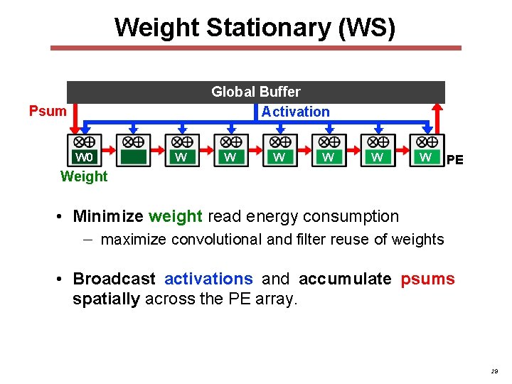
Weight Stationary (WS) Global Buffer Activation Psum W 0 Weight W 1 W 2 W 3 W 4 W 5 W 6 W 7 PE • Minimize weight read energy consumption − maximize convolutional and filter reuse of weights • Broadcast activations and accumulate psums spatially across the PE array. 29

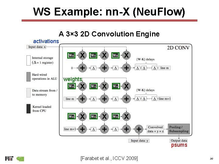
WS Example: nn-X (Neu. Flow) A 3× 3 2 D Convolution Engine activations weights psums [Farabet et al. , ICCV 2009] 30

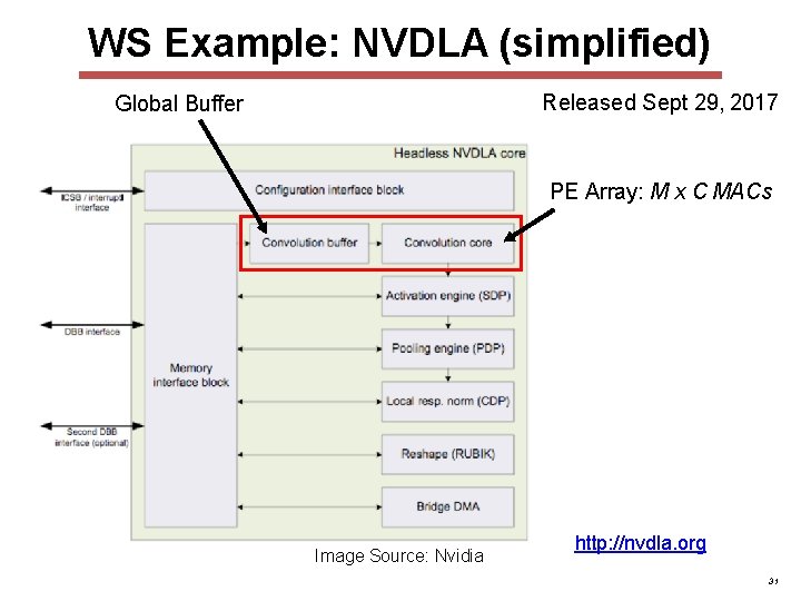
WS Example: NVDLA (simplified) Released Sept 29, 2017 Global Buffer PE Array: M x C MACs Image Source: Nvidia http: //nvdla. org 31

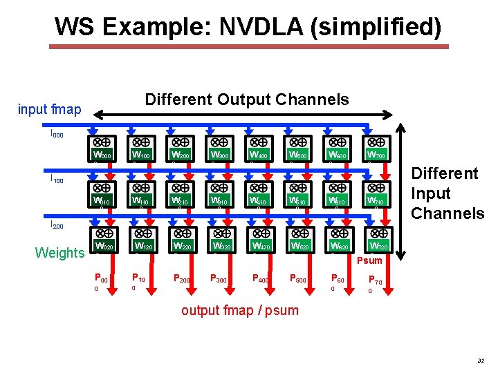
WS Example: NVDLA (simplified) Different Output Channels input fmap I 000 W 100 W 200 W 300 W 400 W 500 W 600 W 700 0 0 0 0 I 100 W 010 W 110 W 210 W 310 W 410 W 510 W 610 W 710 0 0 0 0 I 200 Weights W 020 W 120 W 220 W 320 W 420 W 520 W 620 0 0 0 P 00 P 10 0 0 P 200 P 300 P 400 P 500 P 60 0 Different Input Channels W 720 0 Psum P 70 0 output fmap / psum 32

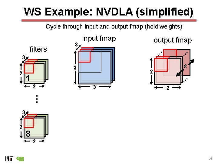
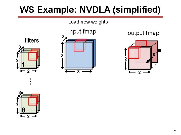
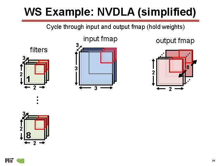
WS Example: NVDLA (simplified) Cycle through input and output fmap (hold weights) output fmap 3 8 2 1 … 2 3 … … filters 3 input fmap 3 2 … 2 3 2 8 2 33

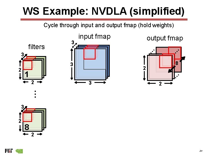
WS Example: NVDLA (simplified) Cycle through input and output fmap (hold weights) output fmap 3 8 2 1 … 2 3 … … filters 3 input fmap 3 2 … 2 3 2 8 2 34

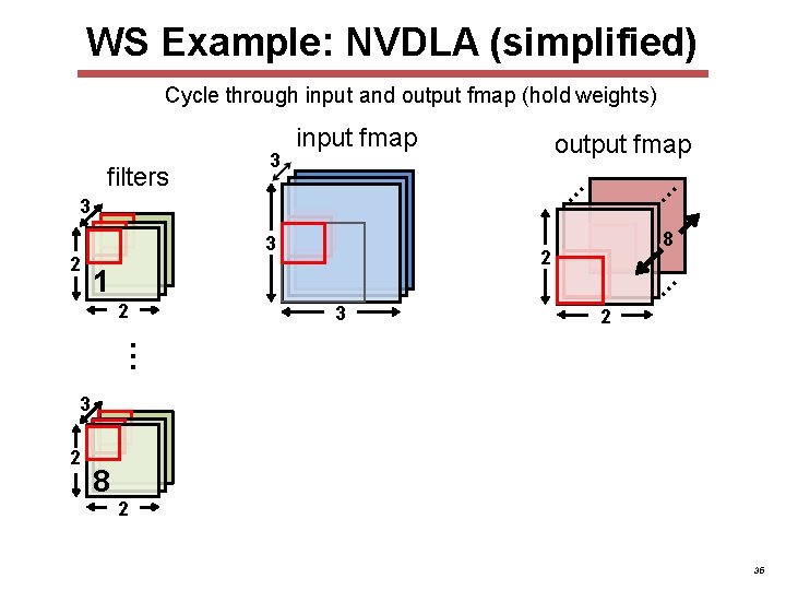
WS Example: NVDLA (simplified) Cycle through input and output fmap (hold weights) output fmap 3 8 2 1 … 2 3 … … filters 3 input fmap 3 2 … 2 3 2 8 2 35

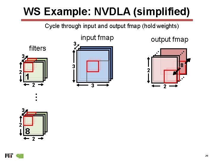
WS Example: NVDLA (simplified) Cycle through input and output fmap (hold weights) output fmap 3 8 2 1 … 2 3 … … filters 3 input fmap 3 2 … 2 3 2 8 2 36

WS Example: NVDLA (simplified) Load new weights output fmap 3 8 2 1 … 2 3 … … filters 3 input fmap 3 2 … 2 3 2 8 2 37

WS Example: NVDLA (simplified) Cycle through input and output fmap (hold weights) output fmap 3 8 2 1 … 2 3 … … filters 3 input fmap 3 2 … 2 3 2 8 2 38

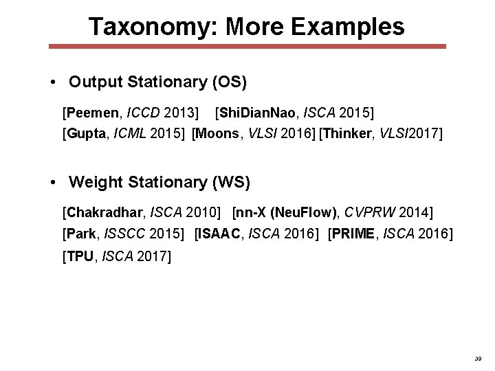
Taxonomy: More Examples • Output Stationary (OS) [Peemen, ICCD 2013] [Shi. Dian. Nao, ISCA 2015] [Gupta, ICML 2015] [Moons, VLSI 2016] [Thinker, VLSI 2017] • Weight Stationary (WS) [Chakradhar, ISCA 2010] [nn-X (Neu. Flow), CVPRW 2014] [Park, ISSCC 2015] [ISAAC, ISCA 2016] [PRIME, ISCA 2016] [TPU, ISCA 2017] 39

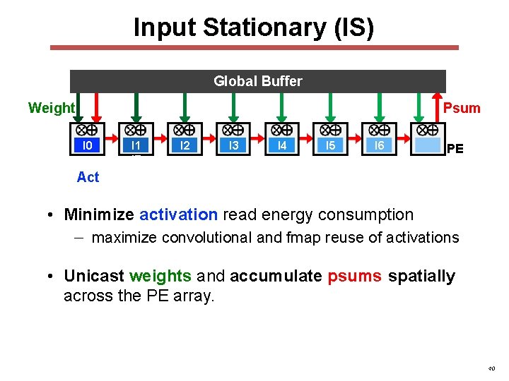
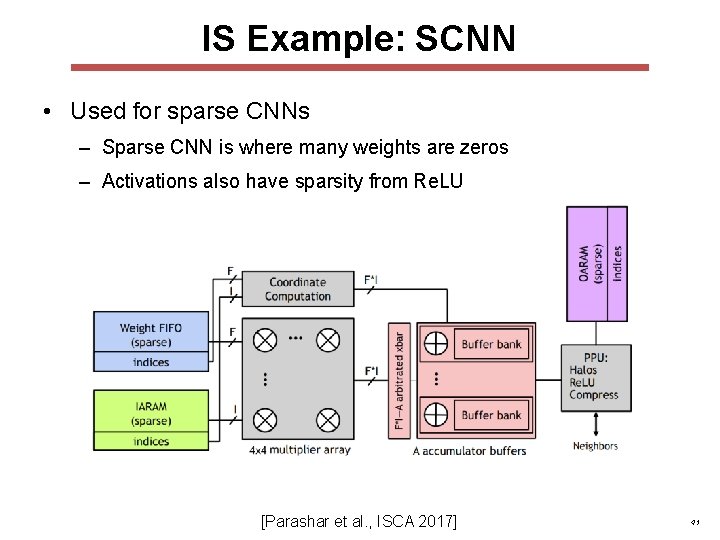
Input Stationary (IS) Global Buffer Weight Psum I 0 I 1 I 7 I 2 I 3 I 4 I 5 I 6 PE Act • Minimize activation read energy consumption − maximize convolutional and fmap reuse of activations • Unicast weights and accumulate psums spatially across the PE array. 40

IS Example: SCNN • Used for sparse CNNs – Sparse CNN is where many weights are zeros – Activations also have sparsity from Re. LU [Parashar et al. , ISCA 2017] 41

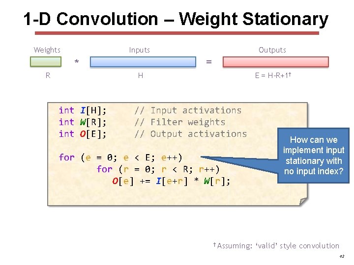
1 -D Convolution – Weight Stationary Weights Inputs = * R Outputs H int I[H]; int W[R]; int O[E]; E = H-R+1† // Input activations // Filter weights // Output activations for (e = 0; e < E; e++) for (r = 0; r < R; r++) O[e] += I[e+r] * W[r]; † Assuming: How can we implement input stationary with no input index? ‘valid’ style convolution 42

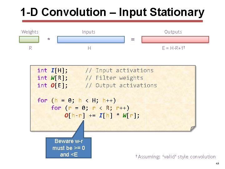
1 -D Convolution – Input Stationary Weights Inputs Outputs = * R H int I[H]; int W[R]; int O[E]; E = H-R+1† // Input activations // Filter weights // Output activations for (h = 0; h < H; h++) for (r = 0; r < R; r++) O[h-r] += I[h] * W[r]; Beware w-r must be >= 0 and <E † Assuming: ‘valid’ style convolution 43

Reference Patterns of Different Dataflows 44

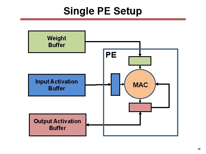
Single PE Setup Weight Buffer PE Input Activation Buffer MAC Output Activation Buffer 45

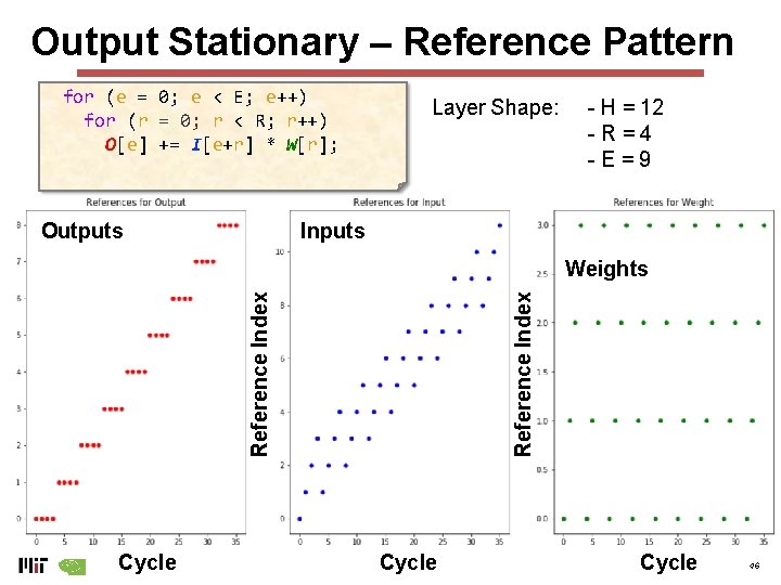
Output Stationary – Reference Pattern for (e = 0; e < E; e++) for (r = 0; r < R; r++) O[e] += I[e+r] * W[r]; Outputs Layer Shape: - H = 12 -R=4 -E=9 Inputs Cycle Reference Index Weights Cycle 46

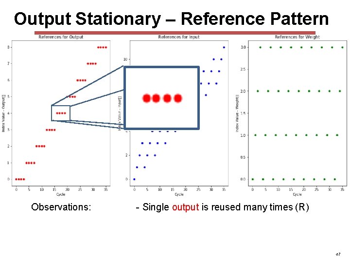
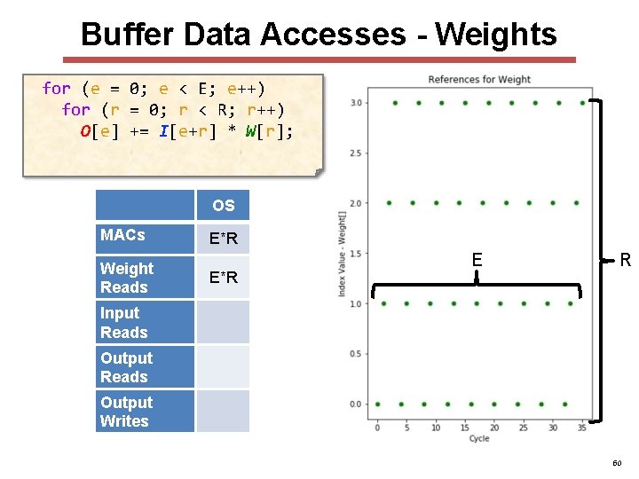
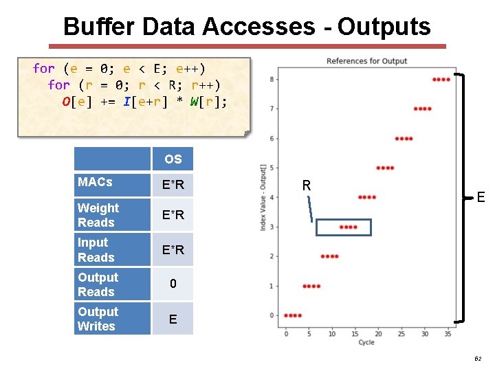
Output Stationary – Reference Pattern Observations: - Single output is reused many times (R) 47

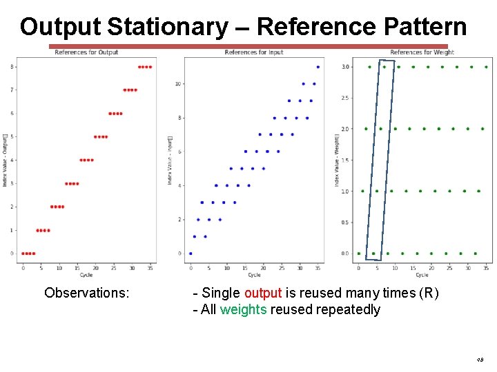
Output Stationary – Reference Pattern Observations: - Single output is reused many times (R) - All weights reused repeatedly 48

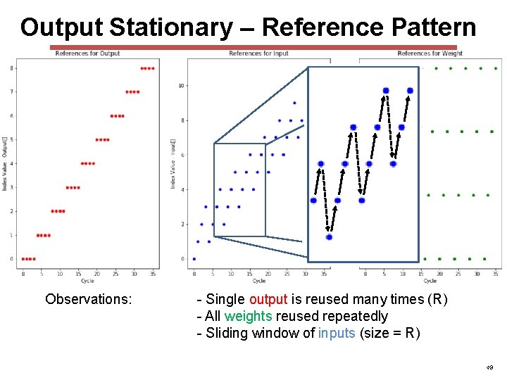
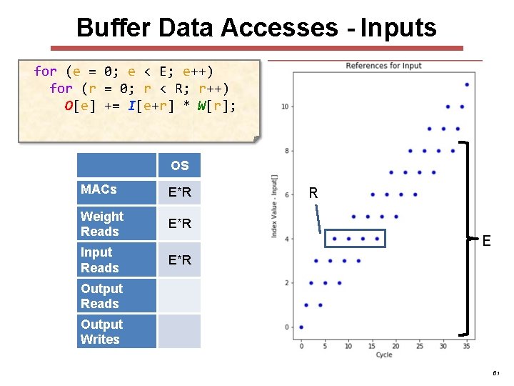
Output Stationary – Reference Pattern Observations: - Single output is reused many times (R) - All weights reused repeatedly - Sliding window of inputs (size = R) 49

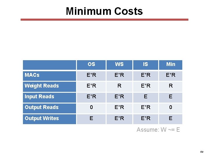
Buffer Data Accesses - Weights for (e = 0; e < E; e++) for (r = 0; r < R; r++) O[e] += I[e+r] * W[r]; OS MACs Weight Reads E*R E R Input Reads Output Writes 50

Buffer Data Accesses - Inputs for (e = 0; e < E; e++) for (r = 0; r < R; r++) O[e] += I[e+r] * W[r]; OS MACs E*R Weight Reads E*R Input Reads E*R R E Output Reads Output Writes 51

Buffer Data Accesses - Outputs for (e = 0; e < E; e++) for (r = 0; r < R; r++) O[e] += I[e+r] * W[r]; OS MACs E*R Weight Reads E*R Input Reads E*R Output Reads 0 Output Writes E R E 52

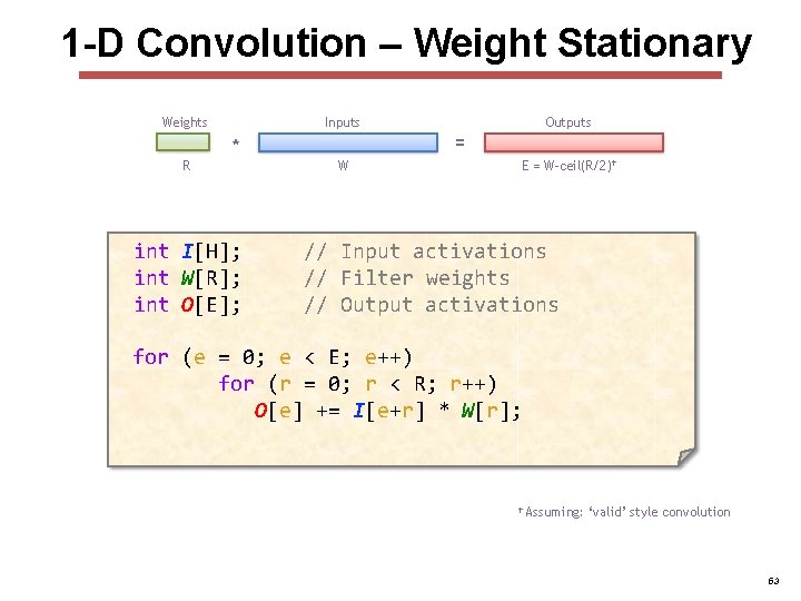
1 -D Convolution – Weight Stationary Weights R Inputs * int I[H]; int W[R]; int O[E]; Outputs = W E = W-ceil(R/2)† // Input activations // Filter weights // Output activations for (e = 0; e < E; e++) for (r = 0; r < R; r++) O[e] += I[e+r] * W[r]; † Assuming: ‘valid’ style convolution 53

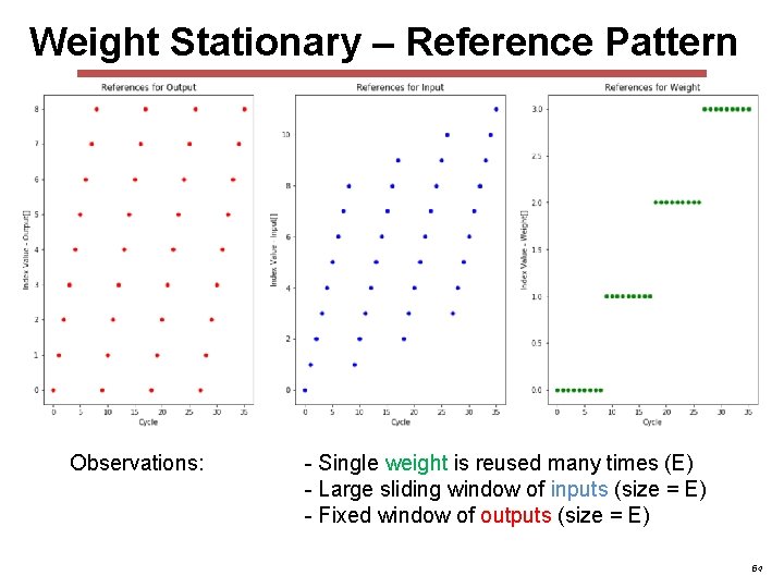
Weight Stationary – Reference Pattern Observations: - Single weight is reused many times (E) - Large sliding window of inputs (size = E) - Fixed window of outputs (size = E) 54

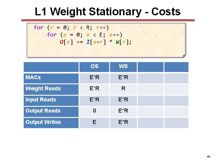
L 1 Weight Stationary - Costs for (r = 0; r < R; r++) for (e = 0; e < E; e++) O[e] += I[e+r] * W[r]; OS WS MACs E*R Weight Reads E*R R Input Reads E*R Output Reads 0 E*R Output Writes E E*R 55

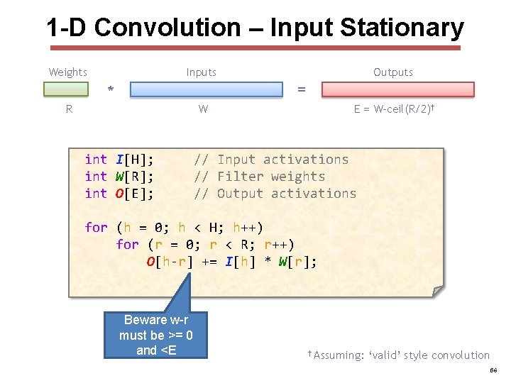
1 -D Convolution – Input Stationary Weights Inputs Outputs = * R W int I[H]; int W[R]; int O[E]; E = W-ceil(R/2)† // Input activations // Filter weights // Output activations for (h = 0; h < H; h++) for (r = 0; r < R; r++) O[h-r] += I[h] * W[r]; Beware w-r must be >= 0 and <E † Assuming: ‘valid’ style convolution 56

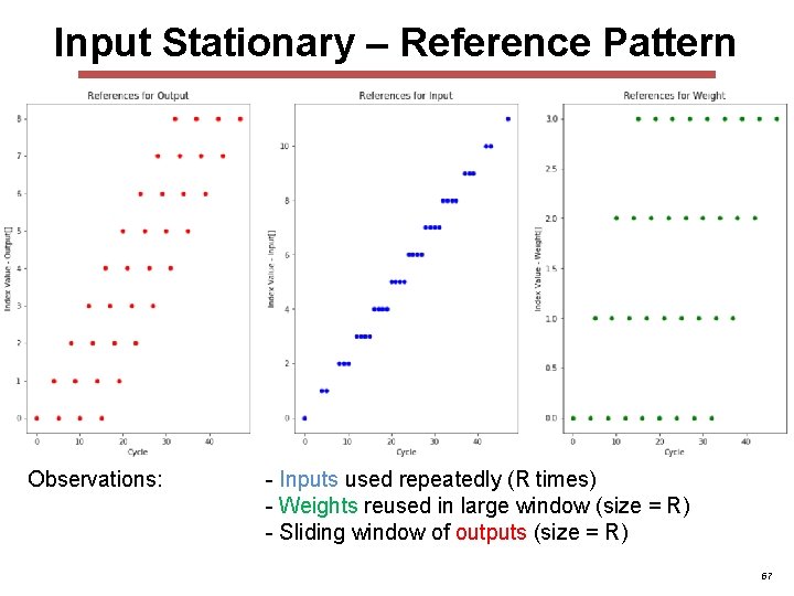
Input Stationary – Reference Pattern Observations: - Inputs used repeatedly (R times) - Weights reused in large window (size = R) - Sliding window of outputs (size = R) 57

Minimum Costs OS WS IS Min MACs E*R E*R Weight Reads E*R R Input Reads E*R E E Output Reads 0 E*R 0 Output Writes E E*R E Assume: W ~= E 58

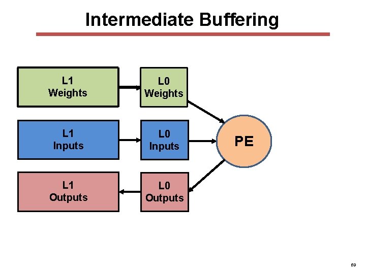
Intermediate Buffering L 1 L 0 Weights L 1 L 0 Inputs L 1 L 0 Outputs PE 59

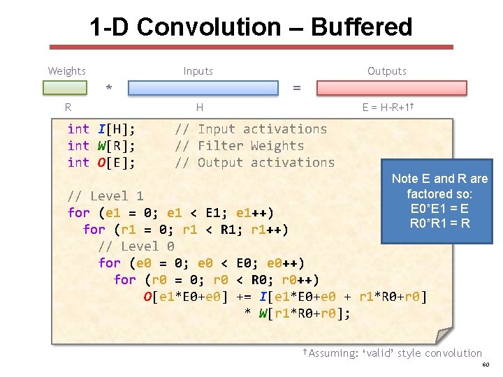
1 -D Convolution – Buffered Weights Inputs = * R int I[H]; int W[R]; int O[E]; Outputs H E = H-R+1† // Input activations // Filter Weights // Output activations Note E and R are factored so: E 0*E 1 = E R 0*R 1 = R // Level 1 for (e 1 = 0; e 1 < E 1; e 1++) for (r 1 = 0; r 1 < R 1; r 1++) // Level 0 for (e 0 = 0; e 0 < E 0; e 0++) for (r 0 = 0; r 0 < R 0; r 0++) O[e 1*E 0+e 0] += I[e 1*E 0+e 0 + r 1*R 0+r 0] * W[r 1*R 0+r 0]; † Assuming: ‘valid’ style convolution 60

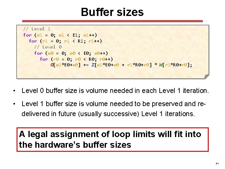
Buffer sizes // Level 1 for (e 1 = 0; e 1 < E 1; e 1++) for (r 1 = 0; r 1 < R 1; r 1++) // Level 0 for (e 0 = 0; e 0 < E 0; e 0++) for (r 0 = 0; r 0 < R 0; r 0++) O[e 1*E 0+e 0] += I[e 1*E 0+e 0 + r 1*R 0+r 0] * W[r 1*R 0+r 0]; • Level 0 buffer size is volume needed in each Level 1 iteration. • Level 1 buffer size is volume needed to be preserved and redelivered in future (usually successive) Level 1 iterations. A legal assignment of loop limits will fit into the hardware’s buffer sizes 61

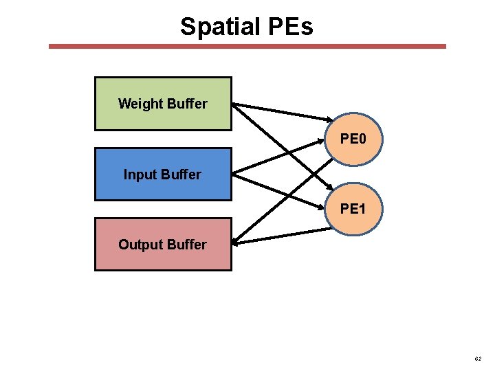
Spatial PEs Weight Buffer PE 0 Input Buffer PE 1 Output Buffer 62

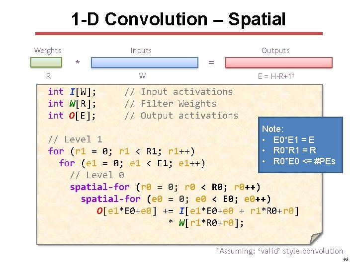
1 -D Convolution – Spatial Weights Inputs = * R int I[W]; int W[R]; int O[E]; Outputs W E = H-R+1† // Input activations // Filter Weights // Output activations Note: • E 0*E 1 = E • R 0*R 1 = R • R 0*E 0 <= #PEs // Level 1 for (r 1 = 0; r 1 < R 1; r 1++) for (e 1 = 0; e 1 < E 1; e 1++) // Level 0 spatial-for (r 0 = 0; r 0 < R 0; r 0++) spatial-for (e 0 = 0; e 0 < E 0; e 0++) O[e 1*E 0+e 0] += I[e 1*E 0+e 0 + r 1*R 0+r 0] * W[r 1*R 0+r 0]; † Assuming: ‘valid’ style convolution 63

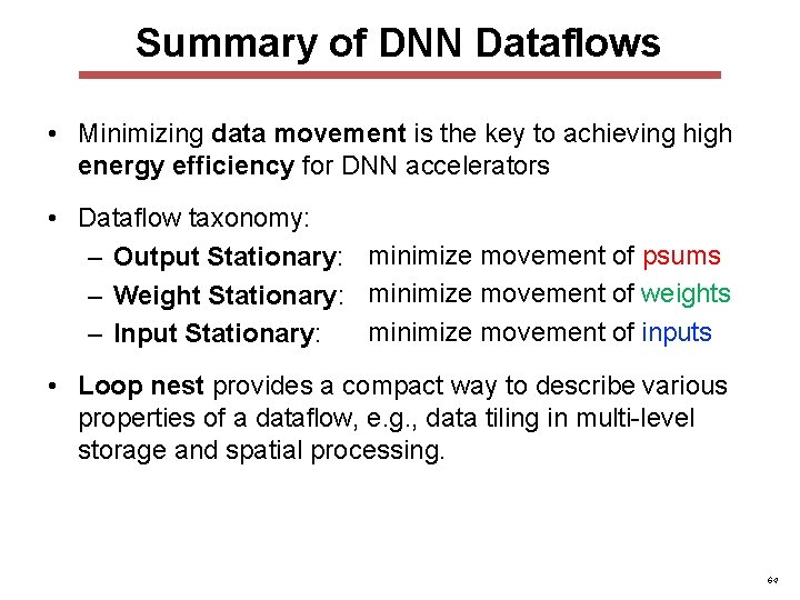
Summary of DNN Dataflows • Minimizing data movement is the key to achieving high energy efficiency for DNN accelerators • Dataflow taxonomy: – Output Stationary: minimize movement of psums – Weight Stationary: minimize movement of weights minimize movement of inputs – Input Stationary: • Loop nest provides a compact way to describe various properties of a dataflow, e. g. , data tiling in multi-level storage and spatial processing. 64