DNA 1 Last weeks takehome lessons Types of

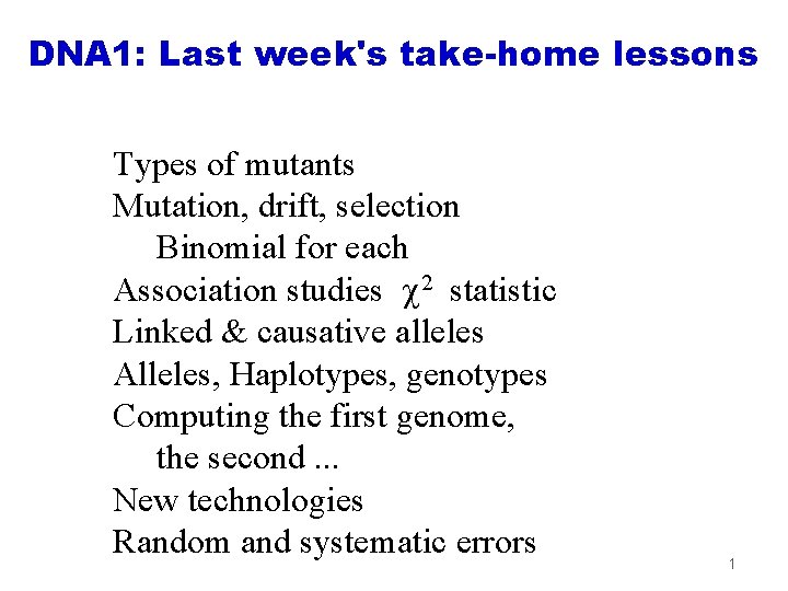
DNA 1: Last week's take-home lessons Types of mutants Mutation, drift, selection Binomial for each Association studies c 2 statistic Linked & causative alleles Alleles, Haplotypes, genotypes Computing the first genome, the second. . . New technologies Random and systematic errors 1

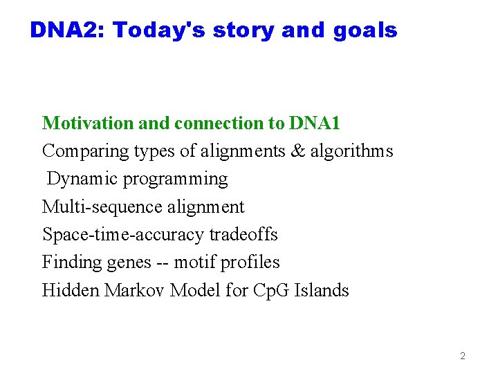
DNA 2: Today's story and goals Motivation and connection to DNA 1 Comparing types of alignments & algorithms Dynamic programming Multi-sequence alignment Space-time-accuracy tradeoffs Finding genes -- motif profiles Hidden Markov Model for Cp. G Islands 2

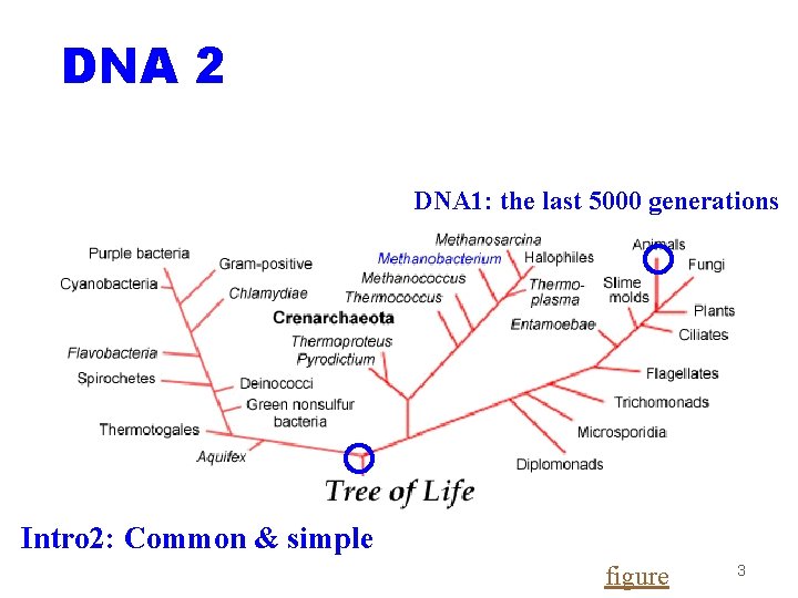
DNA 2 DNA 1: the last 5000 generations Intro 2: Common & simple figure 3

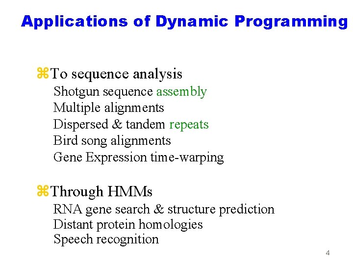
Applications of Dynamic Programming z. To sequence analysis Shotgun sequence assembly Multiple alignments Dispersed & tandem repeats Bird song alignments Gene Expression time-warping z. Through HMMs RNA gene search & structure prediction Distant protein homologies Speech recognition 4

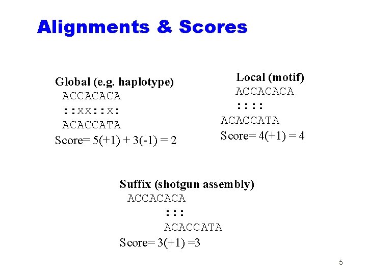
Alignments & Scores Global (e. g. haplotype) ACCACACA : : xx: : x: ACACCATA Score= 5(+1) + 3(-1) = 2 Local (motif) ACCACACA : : ACACCATA Score= 4(+1) = 4 Suffix (shotgun assembly) ACCACACA : : : ACACCATA Score= 3(+1) =3 5

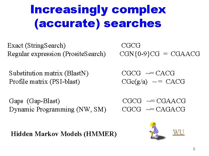
Increasingly complex (accurate) searches Exact (String. Search) Regular expression (Prosite. Search) CGCG CGN{0 -9}CG = CGAACG Substitution matrix (Blast. N) Profile matrix (PSI-blast) CGCG ~= CACG CGc(g/a) ~ = CACG Gaps (Gap-Blast) Dynamic Programming (NW, SM) CGCG ~= CGAACG CGCG ~= CAGACG Hidden Markov Models (HMMER) WU 6

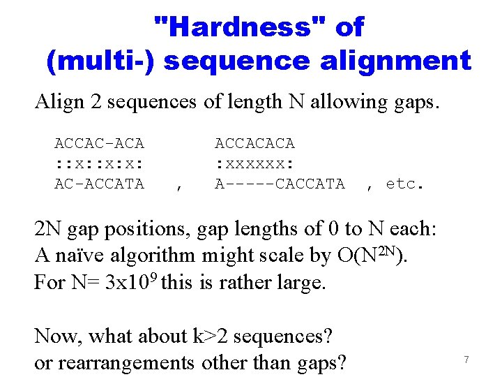
"Hardness" of (multi-) sequence alignment Align 2 sequences of length N allowing gaps. ACCAC-ACA : : x: x: AC-ACCATA , ACCACACA : xxxxxx: A-----CACCATA , etc. 2 N gap positions, gap lengths of 0 to N each: A naïve algorithm might scale by O(N 2 N). For N= 3 x 109 this is rather large. Now, what about k>2 sequences? or rearrangements other than gaps? 7

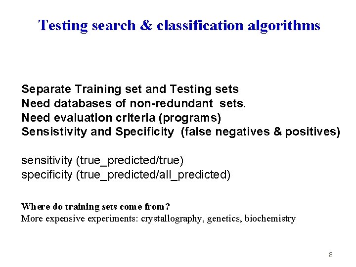
Testing search & classification algorithms Separate Training set and Testing sets Need databases of non-redundant sets. Need evaluation criteria (programs) Sensistivity and Specificity (false negatives & positives) sensitivity (true_predicted/true) specificity (true_predicted/all_predicted) Where do training sets come from? More expensive experiments: crystallography, genetics, biochemistry 8

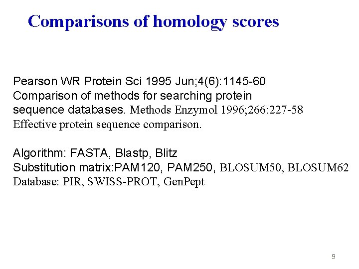
Comparisons of homology scores Pearson WR Protein Sci 1995 Jun; 4(6): 1145 -60 Comparison of methods for searching protein sequence databases. Methods Enzymol 1996; 266: 227 -58 Effective protein sequence comparison. Algorithm: FASTA, Blastp, Blitz Substitution matrix: PAM 120, PAM 250, BLOSUM 62 Database: PIR, SWISS-PROT, Gen. Pept 9

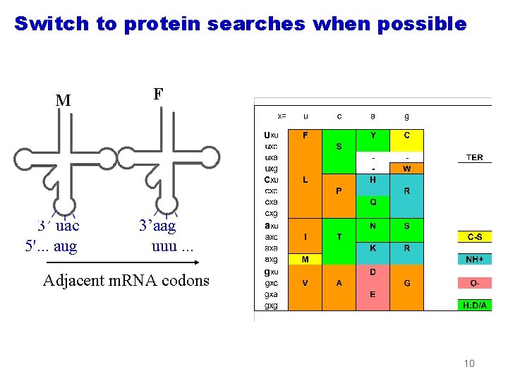
Switch to protein searches when possible M 3’ uac 5'. . . aug F 3’aag uuu. . . Adjacent m. RNA codons 10

A Multiple Alignment of Immunoglobulins 11

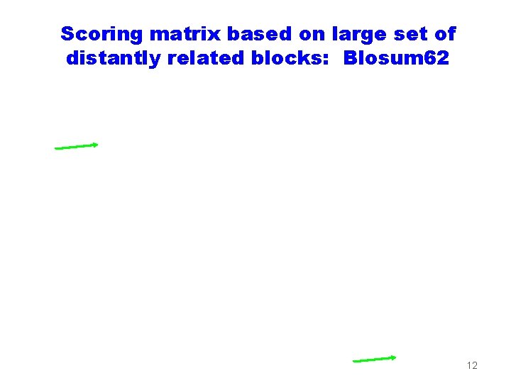
Scoring matrix based on large set of distantly related blocks: Blosum 62 12

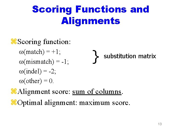
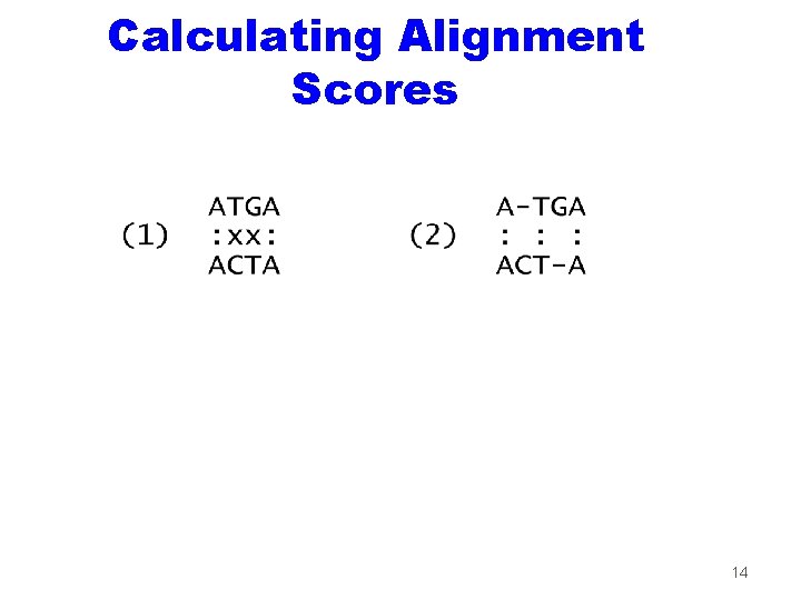
Scoring Functions and Alignments z. Scoring function: (match) = +1; (mismatch) = -1; (indel) = -2; (other) = 0. } substitution matrix z. Alignment score: sum of columns. z. Optimal alignment: maximum score. 13

Calculating Alignment Scores 14

DNA 2: Today's story and goals Motivation and connection to DNA 1 Comparing types of alignments & algorithms Dynamic programming Multi-sequence alignment Space-time-accuracy tradeoffs Finding genes -- motif profiles Hidden Markov Model for Cp. G Islands 15

What is dynamic programming? A dynamic programming algorithm solves every subsubproblem just once and then saves its answer in a table, avoiding the work of recomputing the answer every time the subsubproblem is encountered. -- Cormen et al. "Introduction to Algorithms", The MIT Press. 16

Recursion of Optimal Global Alignments 17

Recursion of Optimal Local Alignments 18

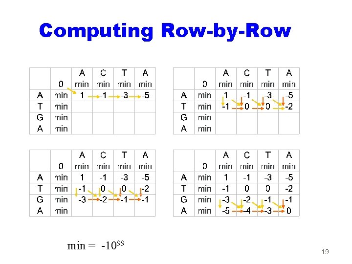
Computing Row-by-Row min = -1099 19

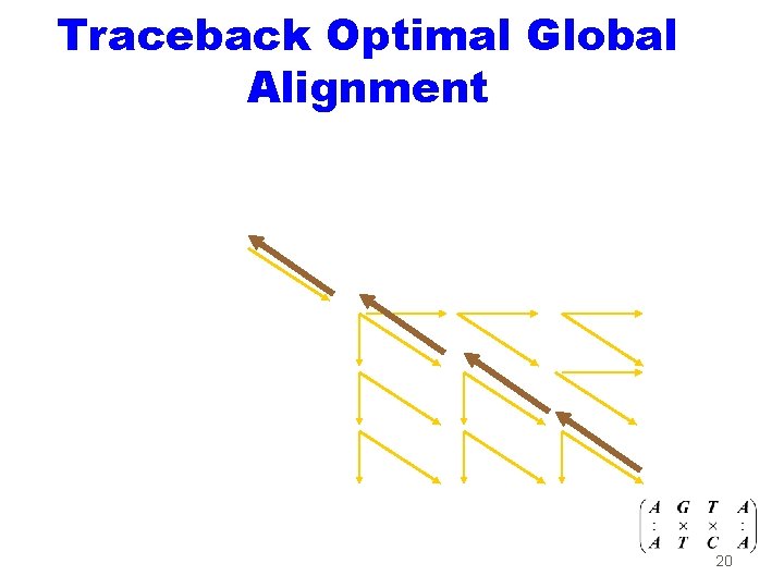
Traceback Optimal Global Alignment 20

Local and Global Alignments 21

Time and Space Complexity of Computing Alignments 22

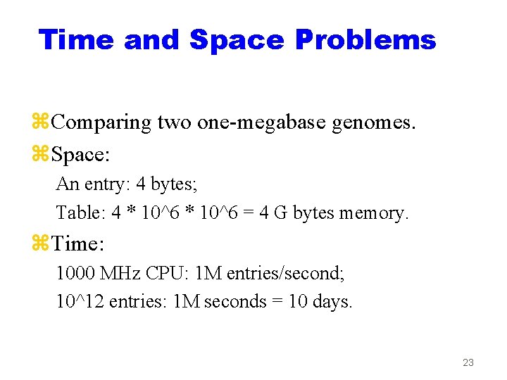
Time and Space Problems z. Comparing two one-megabase genomes. z. Space: An entry: 4 bytes; Table: 4 * 10^6 = 4 G bytes memory. z. Time: 1000 MHz CPU: 1 M entries/second; 10^12 entries: 1 M seconds = 10 days. 23

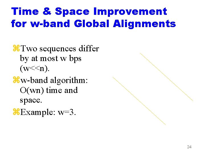
Time & Space Improvement for w-band Global Alignments z. Two sequences differ by at most w bps (w<<n). zw-band algorithm: O(wn) time and space. z. Example: w=3. 24

Summary Dynamic programming Statistical interpretation of alignments Computing optimal global alignment Computing optimal local alignment Time and space complexity Improvement of time and space Scoring functions 25

DNA 2: Today's story and goals Motivation and connection to DNA 1 Comparing types of alignments & algorithms Dynamic programming Multi-sequence alignment Space-time-accuracy tradeoffs Finding genes -- motif profiles Hidden Markov Model for Cp. G Islands 26

A Multiple Alignment of Immunoglobulins 27

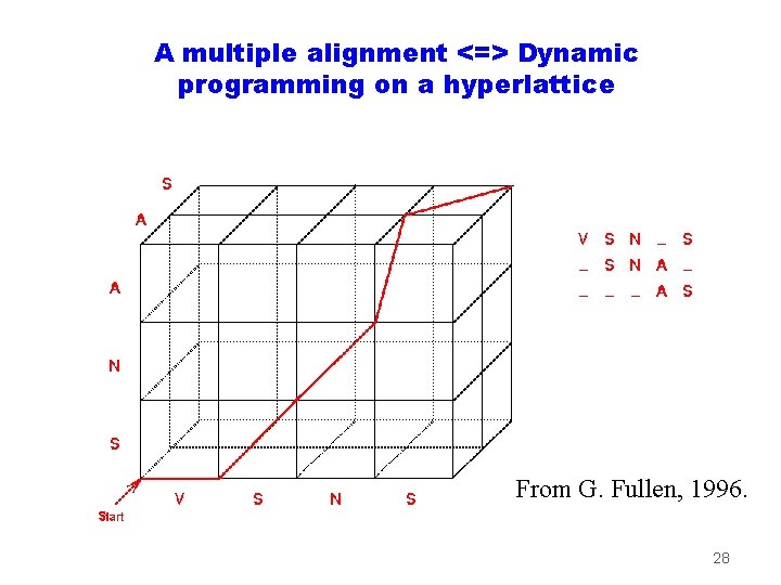
A multiple alignment <=> Dynamic programming on a hyperlattice From G. Fullen, 1996. 28

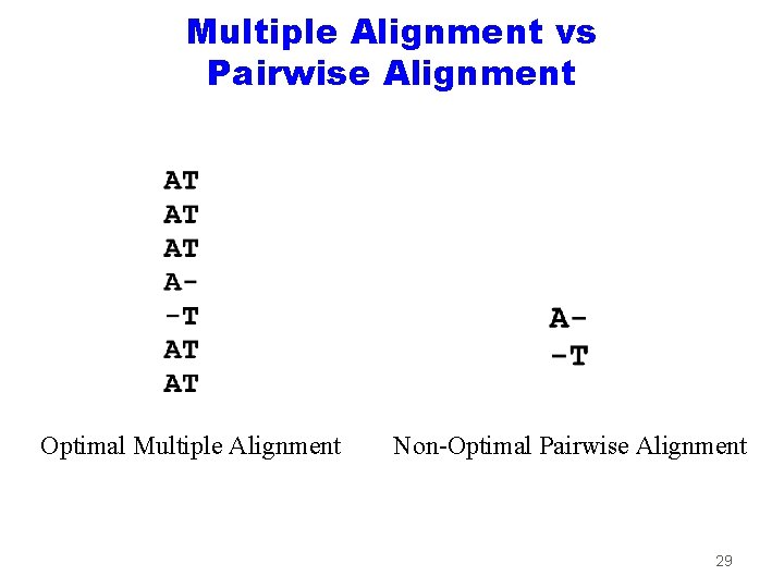
Multiple Alignment vs Pairwise Alignment Optimal Multiple Alignment Non-Optimal Pairwise Alignment 29

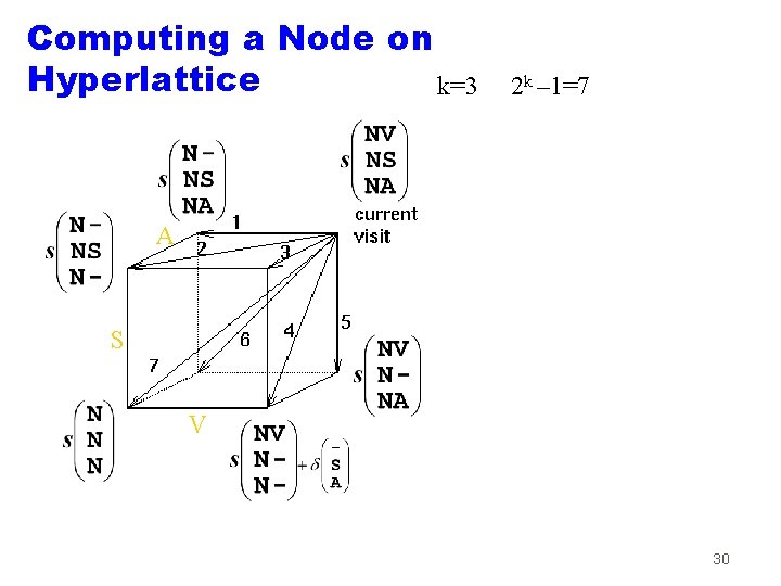
Computing a Node on Hyperlattice k=3 2 k – 1=7 A S V 30

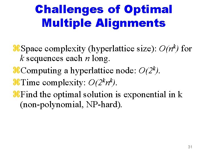
Challenges of Optimal Multiple Alignments z. Space complexity (hyperlattice size): O(nk) for k sequences each n long. z. Computing a hyperlattice node: O(2 k). z. Time complexity: O(2 knk). z. Find the optimal solution is exponential in k (non-polynomial, NP-hard). 31

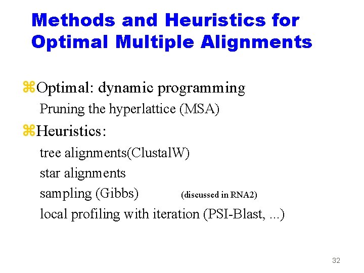
Methods and Heuristics for Optimal Multiple Alignments z. Optimal: dynamic programming Pruning the hyperlattice (MSA) z. Heuristics: tree alignments(Clustal. W) star alignments sampling (Gibbs) (discussed in RNA 2) local profiling with iteration (PSI-Blast, . . . ) 32

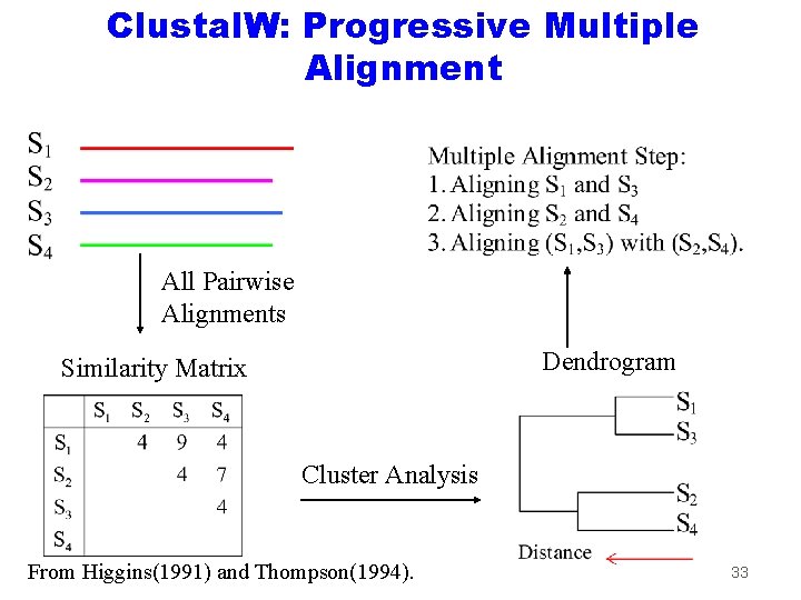
Clustal. W: Progressive Multiple Alignment All Pairwise Alignments Dendrogram Similarity Matrix Cluster Analysis From Higgins(1991) and Thompson(1994). 33

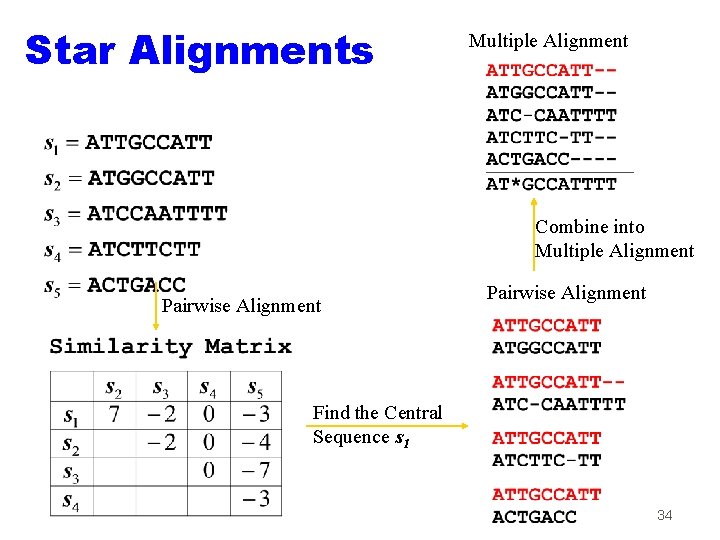
Star Alignments Multiple Alignment Combine into Multiple Alignment Pairwise Alignment Find the Central Sequence s 1 34

DNA 2: Today's story and goals Motivation and connection to DNA 1 Comparing types of alignments & algorithms Dynamic programming Multi-sequence alignment Space-time-accuracy tradeoffs Finding genes -- motif profiles Hidden Markov Model for Cp. G Islands 35

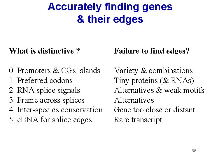
Accurately finding genes & their edges What is distinctive ? Failure to find edges? 0. Promoters & CGs islands 1. Preferred codons 2. RNA splice signals 3. Frame across splices 4. Inter-species conservation 5. c. DNA for splice edges Variety & combinations Tiny proteins (& RNAs) Alternatives & weak motifs Alternatives Gene too close or distant Rare transcript 36

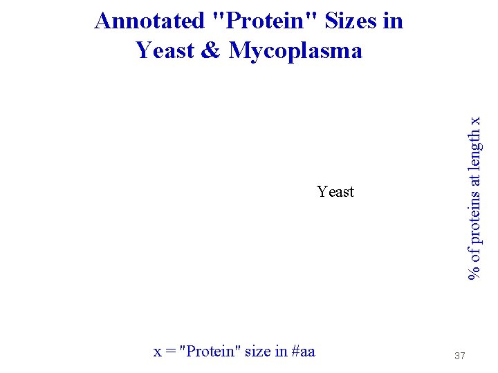
Yeast x = "Protein" size in #aa % of proteins at length x Annotated "Protein" Sizes in Yeast & Mycoplasma 37

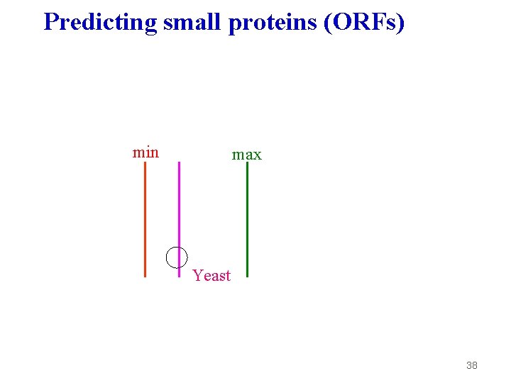
Predicting small proteins (ORFs) min max Yeast 38

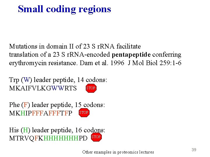
Small coding regions Mutations in domain II of 23 S r. RNA facilitate translation of a 23 S r. RNA-encoded pentapeptide conferring erythromycin resistance. Dam et al. 1996 J Mol Biol 259: 1 -6 Trp (W) leader peptide, 14 codons: MKAIFVLKGWWRTS STOP Phe (F) leader peptide, 15 codons: MKHIPFFFAFFFTFP STOP His (H) leader peptide, 16 codons: MTRVQFKHHHHHHHPD STOP Other examples in proteomics lectures 39

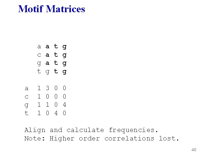
Motif Matrices a c g t a a a g t t g g 1 1 3 0 1 0 0 4 0 Align and calculate frequencies. Note: Higher order correlations lost. 40

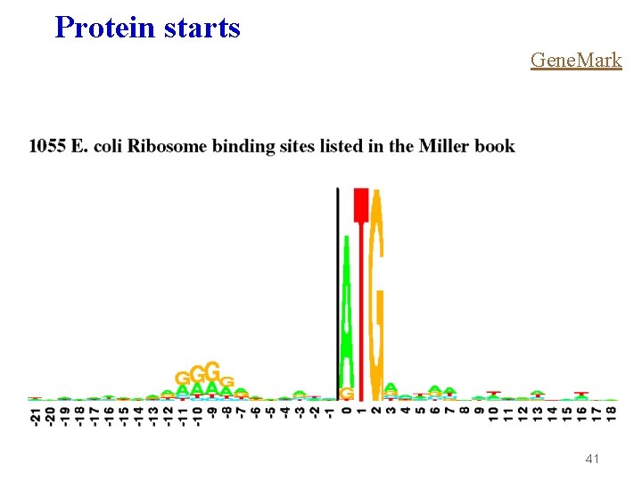
Protein starts Gene. Mark 41

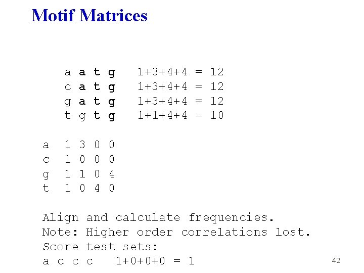
Motif Matrices a c g t a a a g t t g g 1 1 3 0 1 0 0 4 0 Align Note: Score a c c 1+3+4+4 1+1+4+4 = = 12 12 12 10 and calculate frequencies. Higher order correlations lost. test sets: c 1+0+0+0 = 1 42

DNA 2: Today's story and goals Motivation and connection to DNA 1 Comparing types of alignments & algorithms Dynamic programming Multi-sequence alignment Space-time-accuracy tradeoffs Finding genes -- motif profiles Hidden Markov Model for Cp. G Islands 43

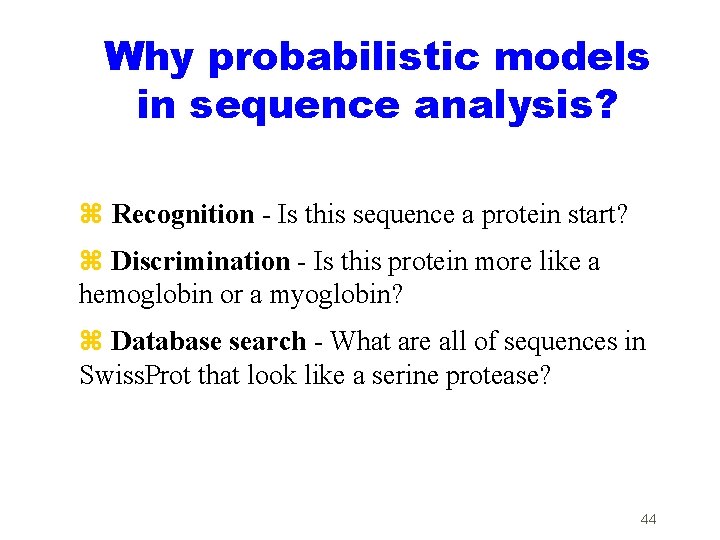
Why probabilistic models in sequence analysis? z Recognition - Is this sequence a protein start? z Discrimination - Is this protein more like a hemoglobin or a myoglobin? z Database search - What are all of sequences in Swiss. Prot that look like a serine protease? 44

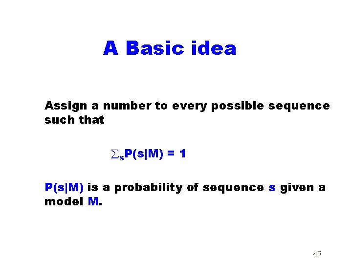
A Basic idea Assign a number to every possible sequence such that s. P(s|M) = 1 P(s|M) is a probability of sequence s given a model M. 45

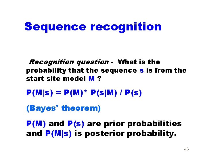
Sequence recognition Recognition question - What is the probability that the sequence s is from the start site model M ? P(M|s) = P(M)* P(s|M) / P(s) (Bayes' theorem) P(M) and P(s) are prior probabilities and P(M|s) is posterior probability. 46

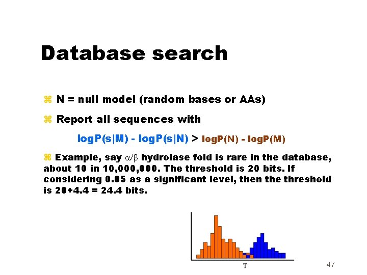
Database search z N = null model (random bases or AAs) z Report all sequences with log. P(s|M) - log. P(s|N) > log. P(N) - log. P(M) z Example, say a/b hydrolase fold is rare in the database, about 10 in 10, 000. The threshold is 20 bits. If considering 0. 05 as a significant level, then the threshold is 20+4. 4 = 24. 4 bits. 47

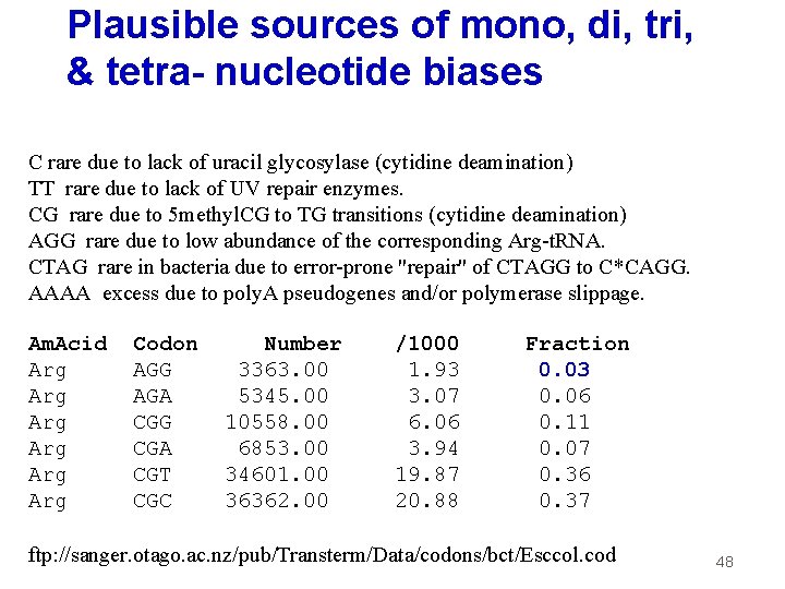
Plausible sources of mono, di, tri, & tetra- nucleotide biases C rare due to lack of uracil glycosylase (cytidine deamination) TT rare due to lack of UV repair enzymes. CG rare due to 5 methyl. CG to TG transitions (cytidine deamination) AGG rare due to low abundance of the corresponding Arg-t. RNA. CTAG rare in bacteria due to error-prone "repair" of CTAGG to C*CAGG. AAAA excess due to poly. A pseudogenes and/or polymerase slippage. Am. Acid Arg Arg Arg Codon AGG AGA CGG CGA CGT CGC Number 3363. 00 5345. 00 10558. 00 6853. 00 34601. 00 36362. 00 /1000 1. 93 3. 07 6. 06 3. 94 19. 87 20. 88 Fraction 0. 03 0. 06 0. 11 0. 07 0. 36 0. 37 ftp: //sanger. otago. ac. nz/pub/Transterm/Data/codons/bct/Esccol. cod 48

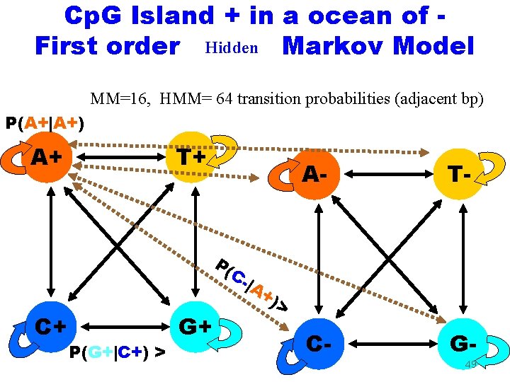
Cp. G Island + in a ocean of First order Hidden Markov Model MM=16, HMM= 64 transition probabilities (adjacent bp) P(A+|A+) A+ T+ P( C+ P(G+|C+) > G+ C|A A- T- C- G- +) > 49

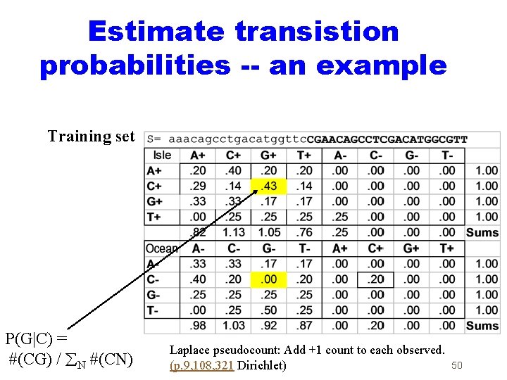
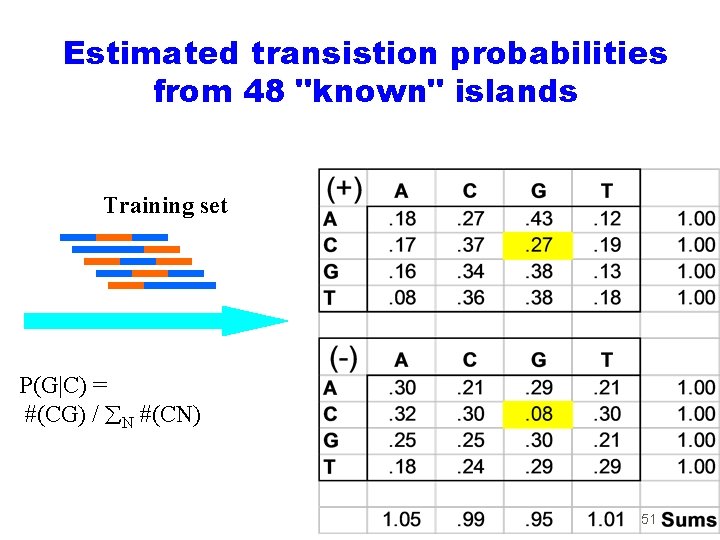
Estimate transistion probabilities -- an example Training set P(G|C) = #(CG) / N #(CN) Laplace pseudocount: Add +1 count to each observed. (p. 9, 108, 321 Dirichlet) 50

Estimated transistion probabilities from 48 "known" islands Training set P(G|C) = #(CG) / N #(CN) 51

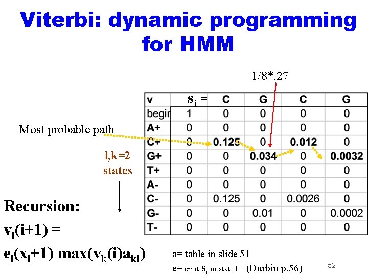
Viterbi: dynamic programming for HMM 1/8*. 27 si = Most probable path l, k=2 states Recursion: vl(i+1) = el(xi+1) max(vk(i)akl) a= table in slide 51 e= emit si in state l (Durbin p. 56) 52

DNA 2: Today's story and goals Motivation and connection to DNA 1 Comparing types of alignments & algorithms Dynamic programming Multi-sequence alignment Space-time-accuracy tradeoffs Finding genes -- motif profiles Hidden Markov Model for Cp. G Islands 53