DMOR DEA Variable Returns to Scale O 7

DMOR DEA
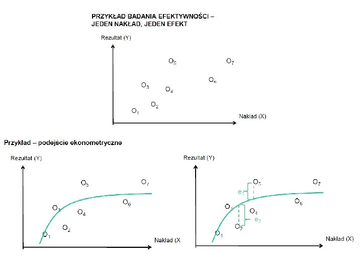

Variable Returns to Scale O 7 O 2 OR O 6 O 3 O 1 O 4 O 2 Constant Returns to Scale

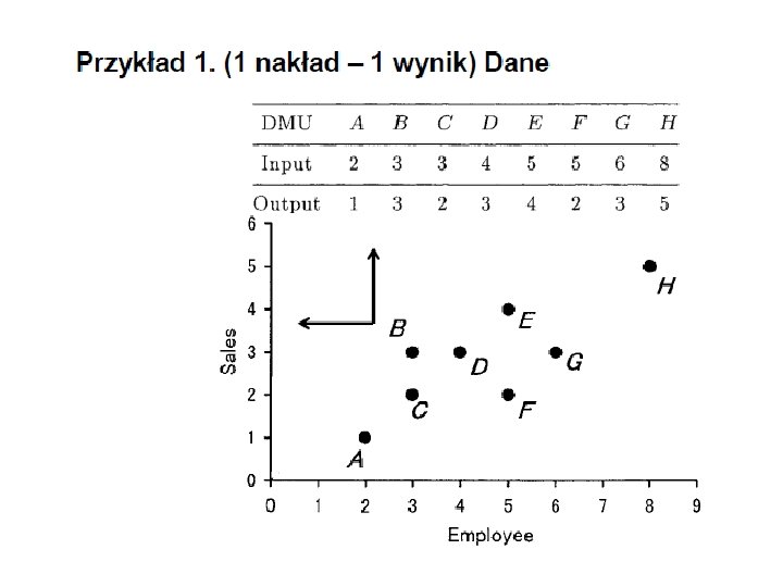
DEA example • For each bank branch we have one output measure and one input measure Branch Croydon Dorking Redhill Reigate Personal No. of transactions ('000) workers 125 18 44 16 80 17 23 11

Efficiency • Inputs are changes into outputs Branch Croydon Dorking Redhill Reigate Personal transactions per worker ('000) 6. 94 2. 75 4. 71 2. 09

Relative efficiency • We can compare all branches relative to Croydon Branch Relative efficiency Croydon Dorking Redhill Reigate =6. 94/6. 94 = 100% =2. 75/6. 94 = 40% =4. 71/6. 94 = 68% =2. 09/6. 94 = 30%
")
More outputs Branch Croydon Dorking Redhill Reigate Personal Business No. of workers transactions ('000) 125 50 18 44 20 16 80 55 17 23 12 11

Efficiency • We now haev two “efficiencies”: Branch Croydon Dorking Redhill Reigate Personal transactions per worker ('000) 6. 94 2. 75 4. 71 2. 09 Business transactions per worker ('000) 2. 78 1. 25 3. 24 1. 09

Graphically

• Reigate – Personal transactions per worker 2090 – Business transactions per worker 1090 – Slope 2090/1090=1. 92

Relative efficiency • Relative efficiency for Reigate • For Reigate = 36% • For Dorking = 43%

Relative efficiency • Technical efficiency – Extended efficiency due to Koopmans, Pareto: • A given entity is fully efficient, if no input and no output can be improved without worsening some other input or output. Dominating entities – Relative efficiency: • A given entity is efficient based on the available evidence, if performance of other entities do not indicate that no input and no output can be improved without worsening some other input or output. • There is no reference to prices and weights of inputs and outputs. • You don’t need to establish the relation between inputs and outputs A desirable direction

capital If we know that there is a technology which enables • producing q 0 units of output • using L units of labor and K units of capital according to the prodction function: Technical efficiency definition: Produce a given level of output using the minimal level of inputs labor capital Then we can measure inefficiency: • e. g. suppose that entity A produces q 0 units of outputs • Then OA’/OA is entity A’s efficiency A A’ O labor

DEA approach E, F, G, H, I is the efficient frontier capital • Production function isoquant is not known directly • DEA estimates it from the data using interval-wise linear interpolation • Assume that firms A, B, C, D, E, F, G, H, I all produce q 0 units of output C E A B F D G H O I labor

DEA efficiency E, F, G, H, I is efficient frontier capital C E A B F G D A’ H O I labor • Efficiency of A according to DEA is OA’/OA • A’ is a shadow or a phantom of A – It is a linear combination of F and G
")
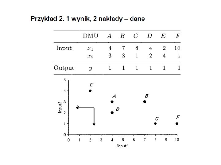
Adding a couple of new branches Business Personal transactions Branch s per worker ('000) Croydon 6. 94 2. 78 Dorking 2. 75 1. 25 Redhill 4. 71 3. 24 Reigate 2. 09 1. 09 A 1. 23 2. 92 B 4. 43 2. 23 C 3. 32 2. 81 D 3. 70 2. 68 E 3. 34 2. 96

Adding branch F • Branch F has 1000 personal transactions per worker • And 6000 business transactions per worker

Adding branch G Branch Croydon Dorking Redhill Reigate A B C D E F G Personal transactions per worker ('000) 6. 94 2. 75 4. 71 2. 09 1. 23 4. 43 3. 32 3. 70 3. 34 1. 00 5. 00 Business transactions per worker ('000) 2. 78 1. 25 3. 24 1. 09 2. 92 2. 23 2. 81 2. 68 2. 96 6. 00 5. 00

The efficient one does not have to win in any category
– primal problem")
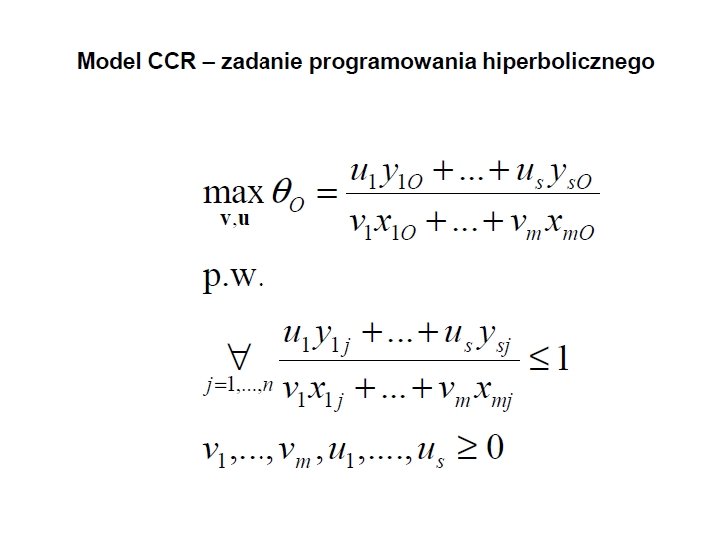
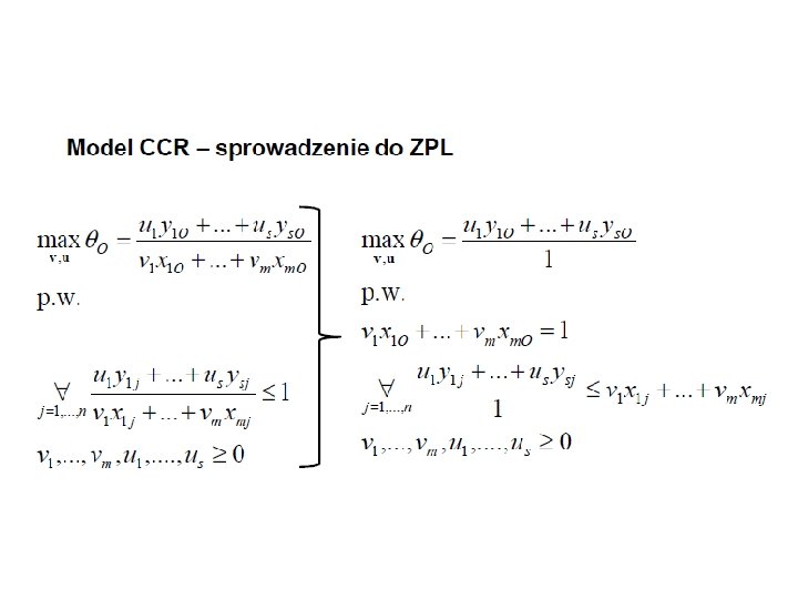
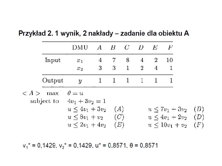
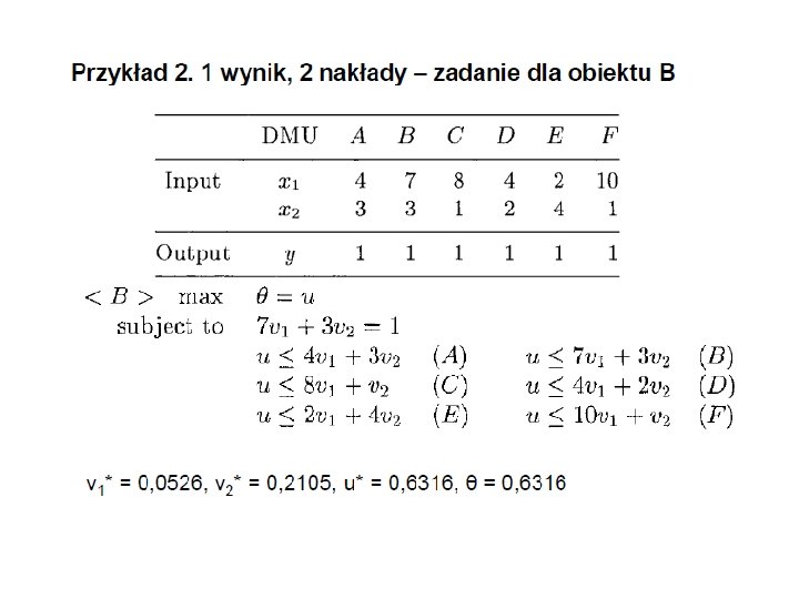
Constant returns to scale (CCR)– primal problem

F is efficient in a weak sense
: decomposition into scale efficiency and")
Constant and Variable returns to scale (CRS i VRS): decomposition into scale efficiency and pure technical efficiency

• Primal problem Multiplier model: • Dual problem: Envelopment model:

• “Strong disposal” assumption – Ignores presence of nonzero slack variables – Different solutions may have nonzero slack variables or not – Therefore one uses 2 phase of the dual problem to maximize these variables (to see whethere exists a solution with nonzero slack variables)

First and second phase of the dual problem may be written together and solved in two steps

Model Input-oriented Output-oriented

Example: Input oriented dual problem for P 5

Input oriented primal problem for P 5

Results

Efficient frontier projection in input oriented model

Efficient frontier projection in output oriented model

Next example
: Dual problem for DMU 5 Variable Returns to")
Model BBC (Variable Returns to Scale): Dual problem for DMU 5 Variable Returns to Scale Technical efficiency for DMU 5 may be reached for DMU 2, which lies on the efficient frontier
 The same problem for DMU 4 gives:")
DMU 4 is weakly DEA efficient 3) The same problem for DMU 4 gives:

How to interpret weights? • Assume that we consider an entity with efficiency less than 1 • Assume that , the rest of the weights are zero • Then the phantom inputs of the entity are: • And the phantom outputs of the entity are:
- Slides: 45