Divide and Conquer The most well known algorithm

Divide and Conquer The most well known algorithm design strategy: 1. Divide instance of problem into two or more smaller instances 2. Solve smaller instances recursively 3. Obtain solution to original (larger) instance by combining these solutions

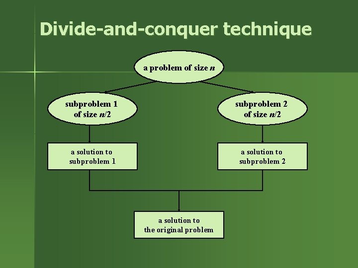
Divide-and-conquer technique a problem of size n subproblem 1 of size n/2 subproblem 2 of size n/2 a solution to subproblem 1 a solution to subproblem 2 a solution to the original problem

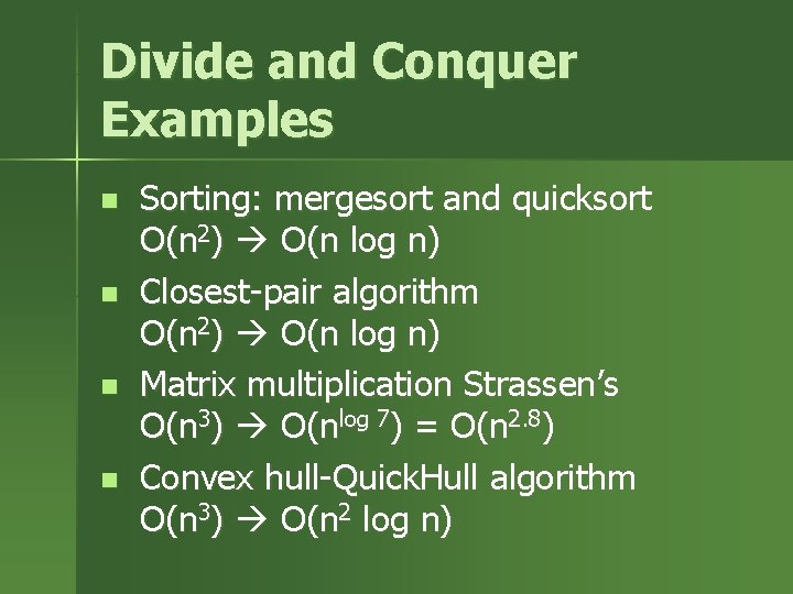
Divide and Conquer Examples n n Sorting: mergesort and quicksort O(n 2) O(n log n) Closest-pair algorithm O(n 2) O(n log n) Matrix multiplication Strassen’s O(n 3) O(nlog 7) = O(n 2. 8) Convex hull-Quick. Hull algorithm O(n 3) O(n 2 log n)

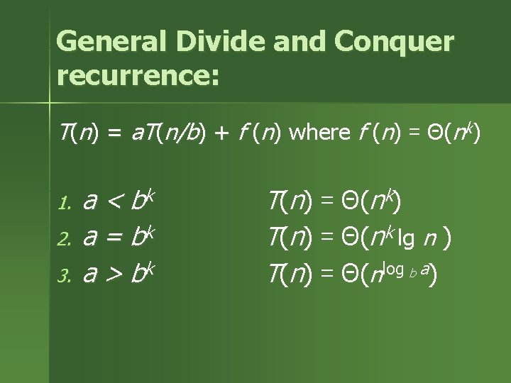
General Divide and Conquer recurrence: T(n) = a. T(n/b) + f (n) where f (n) = Θ(nk) 1. 2. 3. a < bk a = bk a > bk T ( n ) = Θ ( n k) T(n) = Θ(nk lg n ) T(n) = Θ(nlog b a)

Efficiency of mergesort n n All cases have same time efficiency: Θ( n log n) Number of comparisons is close to theoretical minimum for comparison-based sorting: log (n !) ≈ n log n - 1. 44 n Space requirement: Θ( n ) (NOT in-place) Can be implemented without recursion (bottom -up)

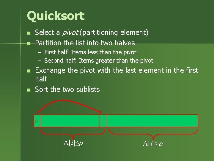
Quicksort n n Select a pivot (partitioning element) Partition the list into two halves – First half: Items less than the pivot – Second half: Items greater than the pivot n n Exchange the pivot with the last element in the first half Sort the two sublists p A[i]≤p A[i]>p

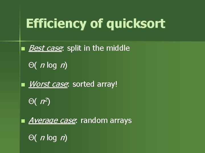
Efficiency of quicksort n Best case: split in the middle Θ( n log n) n Worst case: sorted array! Θ( n 2) n Average case: random arrays Θ( n log n)

Efficiency of quicksort n n Improvements: – better pivot selection: median of three partitioning avoids worst case in sorted files – switch to insertion sort on small subfiles – elimination of recursion these combine to 20 -25% improvement Considered the method of choice for internal sorting for large files (n ≥ 10000)

Efficiency of Quick. Hull algorithm n n If points are not initially sorted by xcoordinate value, this can be accomplished in Θ( n log n) — no increase in asymptotic efficiency class Other algorithms for convex hull: – Graham’s scan – DCHull also in Θ( n log n)

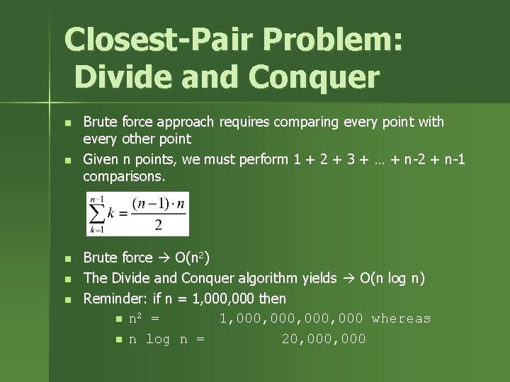
Closest-Pair Problem: Divide and Conquer n n n Brute force approach requires comparing every point with every other point Given n points, we must perform 1 + 2 + 3 + … + n-2 + n-1 comparisons. Brute force O(n 2) The Divide and Conquer algorithm yields O(n log n) Reminder: if n = 1, 000 then n n 2 = 1, 000, 000 whereas n n log n = 20, 000

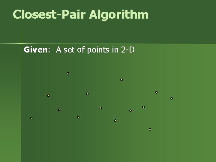
Closest-Pair Algorithm Given: A set of points in 2 -D

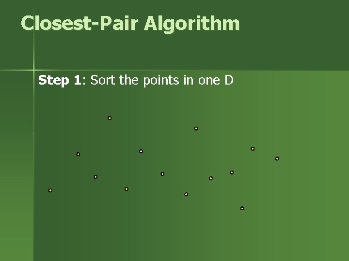
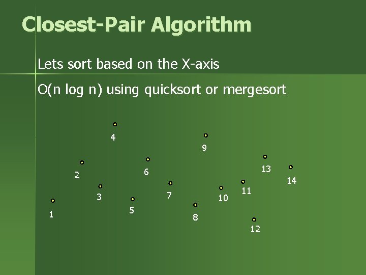
Closest-Pair Algorithm Step 1: Sort the points in one D

Closest-Pair Algorithm Lets sort based on the X-axis O(n log n) using quicksort or mergesort 4 9 7 3 1 13 6 2 5 10 11 8 12 14

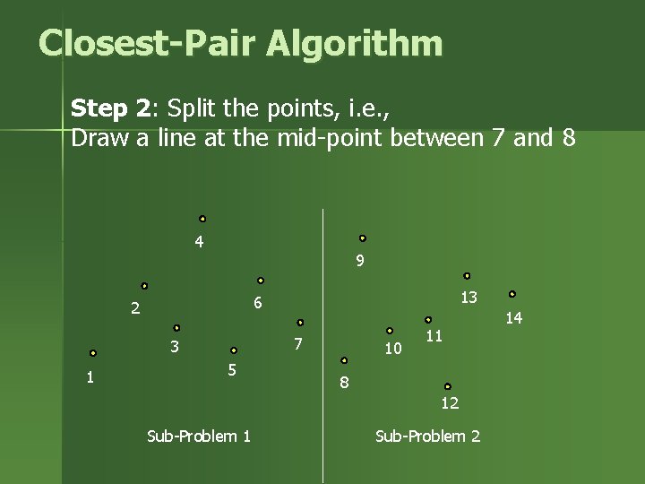
Closest-Pair Algorithm Step 2: Split the points, i. e. , Draw a line at the mid-point between 7 and 8 4 9 7 3 1 13 6 2 5 10 11 8 12 Sub-Problem 1 Sub-Problem 2 14

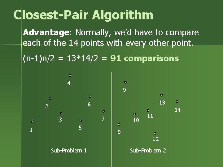
Closest-Pair Algorithm Advantage: Normally, we’d have to compare each of the 14 points with every other point. (n-1)n/2 = 13*14/2 = 91 comparisons 4 9 7 3 1 13 6 2 5 10 11 8 12 Sub-Problem 1 Sub-Problem 2 14

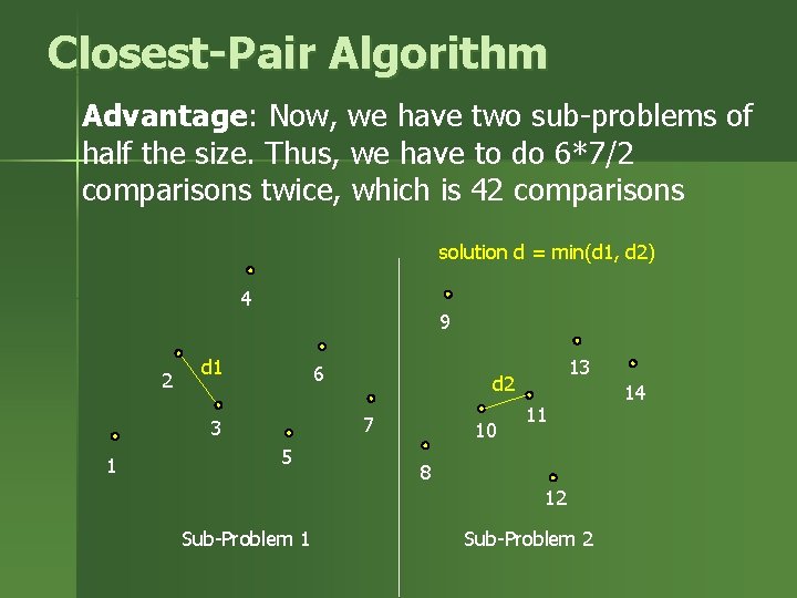
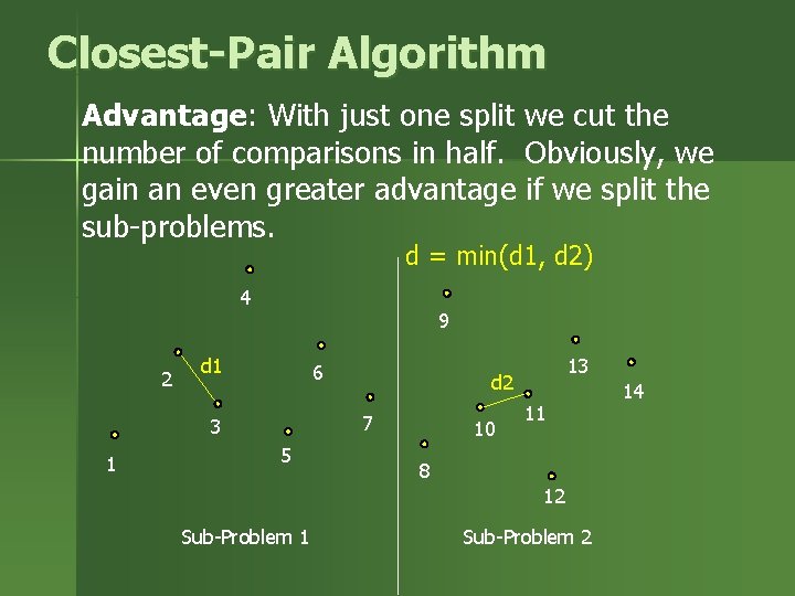
Closest-Pair Algorithm Advantage: Now, we have two sub-problems of half the size. Thus, we have to do 6*7/2 comparisons twice, which is 42 comparisons solution d = min(d 1, d 2) 4 2 9 d 1 6 1 d 2 7 3 5 13 10 11 8 12 Sub-Problem 1 Sub-Problem 2 14

Closest-Pair Algorithm Advantage: With just one split we cut the number of comparisons in half. Obviously, we gain an even greater advantage if we split the sub-problems. d = min(d 1, d 2) 4 2 9 d 1 6 1 d 2 7 3 5 13 10 11 8 12 Sub-Problem 1 Sub-Problem 2 14

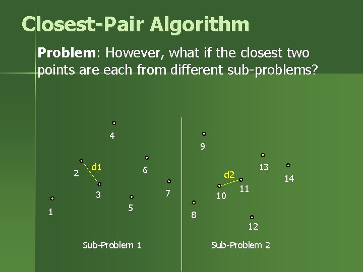
Closest-Pair Algorithm Problem: However, what if the closest two points are each from different sub-problems? 4 2 9 d 1 6 1 d 2 7 3 5 13 10 11 8 12 Sub-Problem 1 Sub-Problem 2 14

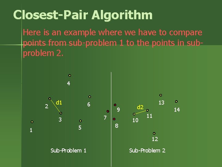
Closest-Pair Algorithm Here is an example where we have to compare points from sub-problem 1 to the points in subproblem 2. 4 2 d 1 6 7 3 1 9 5 8 13 d 2 10 11 12 Sub-Problem 1 Sub-Problem 2 14

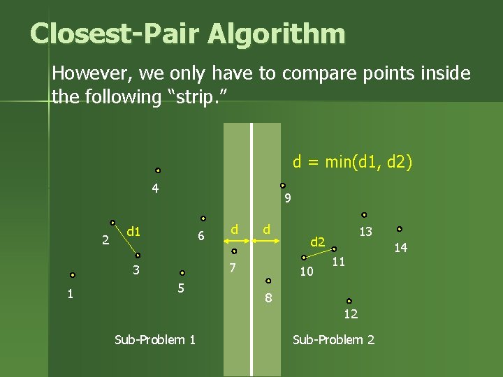
Closest-Pair Algorithm However, we only have to compare points inside the following “strip. ” d = min(d 1, d 2) 4 2 9 d 1 6 d 7 3 1 d 5 13 d 2 10 11 8 12 Sub-Problem 1 Sub-Problem 2 14

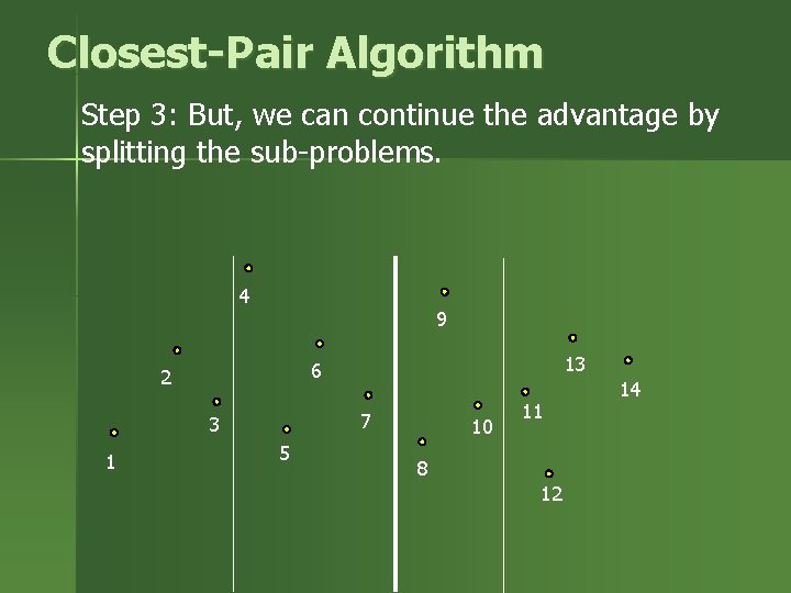
Closest-Pair Algorithm Step 3: But, we can continue the advantage by splitting the sub-problems. 4 9 7 3 1 13 6 2 5 10 11 8 12 14

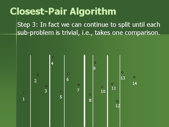
Closest-Pair Algorithm Step 3: In fact we can continue to split until each sub-problem is trivial, i. e. , takes one comparison. 4 9 7 3 1 13 6 2 5 10 11 8 12 14

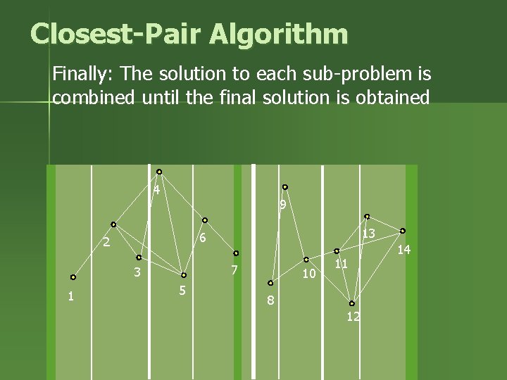
Closest-Pair Algorithm Finally: The solution to each sub-problem is combined until the final solution is obtained 4 9 7 3 1 13 6 2 5 10 11 8 12 14

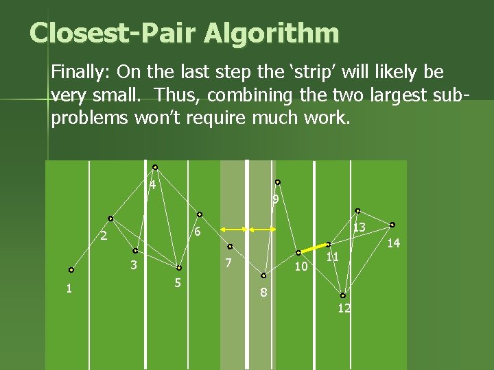
Closest-Pair Algorithm Finally: On the last step the ‘strip’ will likely be very small. Thus, combining the two largest subproblems won’t require much work. 4 9 7 3 1 13 6 2 5 10 11 8 12 14

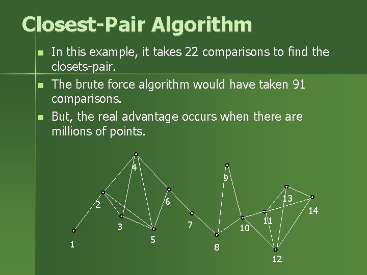
Closest-Pair Algorithm n n n In this example, it takes 22 comparisons to find the closets-pair. The brute force algorithm would have taken 91 comparisons. But, the real advantage occurs when there are millions of points. 4 9 7 3 1 13 6 2 5 10 11 8 12 14

Closest-Pair Problem: Divide and Conquer n n Here is another animation: http: //www. cs. mcgill. ca/~cs 251/Closest. Pair/Close st. Pair. Applet/Closest. Pair. Applet. html