Divide and Conquer and Noncomparisonbased Sorting Algorithms Textbook

Divide and Conquer and Noncomparison-based Sorting Algorithms Textbook: Sedgewick Chapters 7 and 8 Sedgewick Chapter 6. 10, Chapter 10 COMP 2521 18 x 1

Exercise What is the time complexity of merging two sorted linked lists together into one sorted linked list?

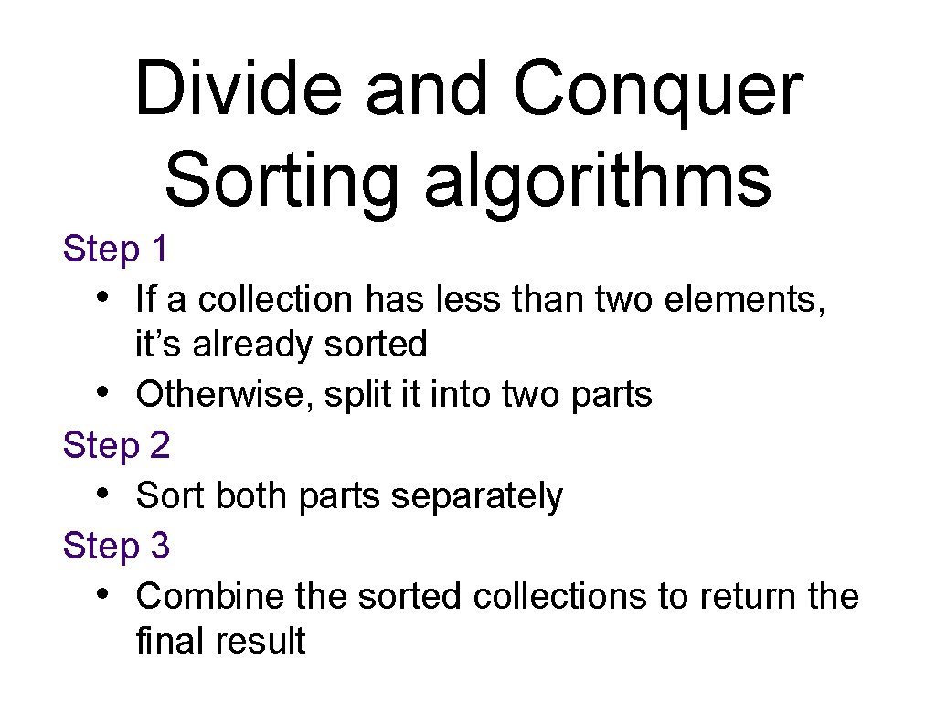
Divide and Conquer Sorting algorithms Step 1 • If a collection has less than two elements, it’s already sorted • Otherwise, split it into two parts Step 2 • Sort both parts separately Step 3 • Combine the sorted collections to return the final result

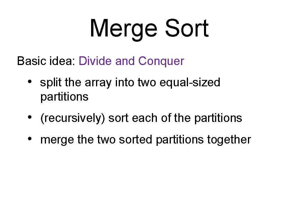
Merge Sort Basic idea: Divide and Conquer • split the array into two equal-sized partitions • (recursively) sort each of the partitions • merge the two sorted partitions together

Merge Sort Merging: Basic idea • copy elements from the inputs one at a time • give preference to the smaller of the two • when one exhausted, copy the rest of the other

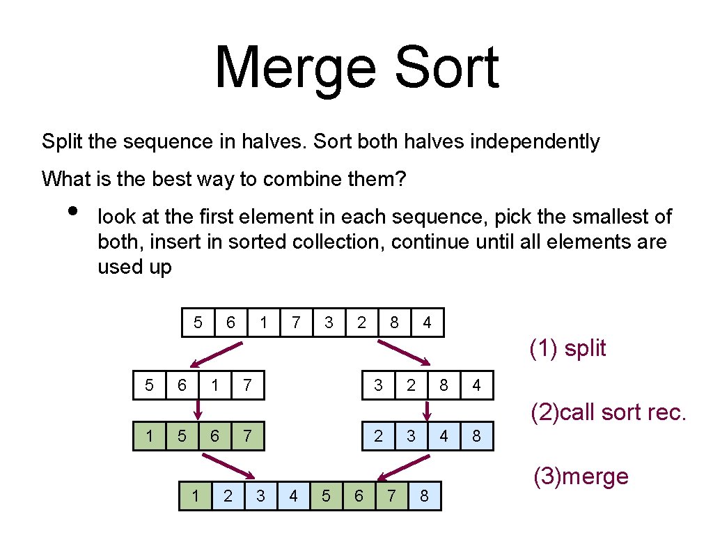
Merge Sort Split the sequence in halves. Sort both halves independently What is the best way to combine them? • look at the first element in each sequence, pick the smallest of both, insert in sorted collection, continue until all elements are used up 5 6 1 7 3 2 8 4 (1) split 5 6 1 7 3 2 8 4 (2)call sort rec. 1 5 6 1 7 2 2 3 4 5 6 3 7 4 8 8 (3)merge

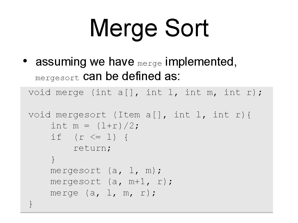
Merge Sort • assuming we have merge implemented, mergesort can be defined as: void merge (int a[], int l, int m, int r); void mergesort (Item a[], int l, int r){ int m = (l+r)/2; if (r <= l) { return; } mergesort (a, l, m); mergesort (a, m+1, r); merge (a, l, m, r); }

Merge Sort void merge(int a[], int l, int mid, int r) { int i, j, k, nitems = r-l+1; int *tmp = malloc(nitems*sizeof(int)); i = l; j = mid+1; k = 0; while (i <= mid && j <= r) { if ( a[i] < a[j] ) { tmp[k++] = a[i++]; }else{ tmp[k++] = a[j++]; } } while (i <= mid) tmp[k++] = a[i++]; while (j <= r) tmp[k++] = a[j++]; //copy back for (i = l, k = 0; i <= r; i++, k++) a[i] = tmp[k]; free(tmp); }

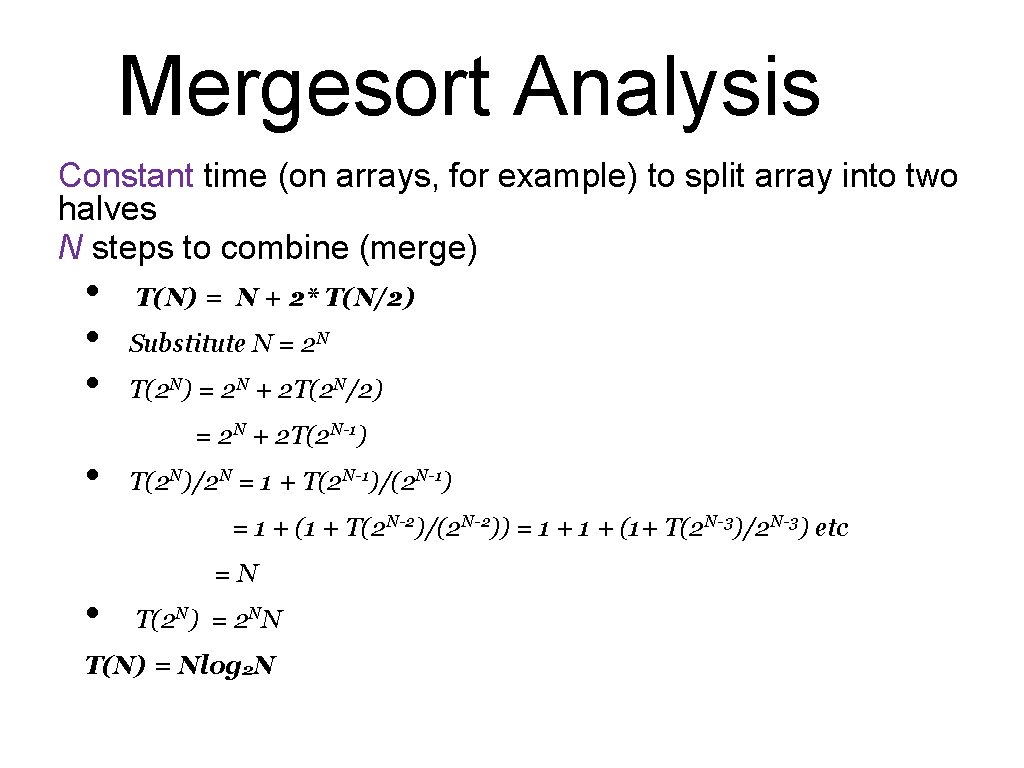
Mergesort Analysis Constant time (on arrays, for example) to split array into two halves N steps to combine (merge) • • T(N) = N + 2* T(N/2) Substitute N = 2 N T(2 N) = 2 N + 2 T(2 N/2) = 2 N + 2 T(2 N-1) T(2 N)/2 N = 1 + T(2 N-1)/(2 N-1) = 1 + (1 + T(2 N-2)/(2 N-2)) = 1 + (1+ T(2 N-3)/2 N-3) etc • =N T(2 N) = 2 NN T(N) = Nlog 2 N

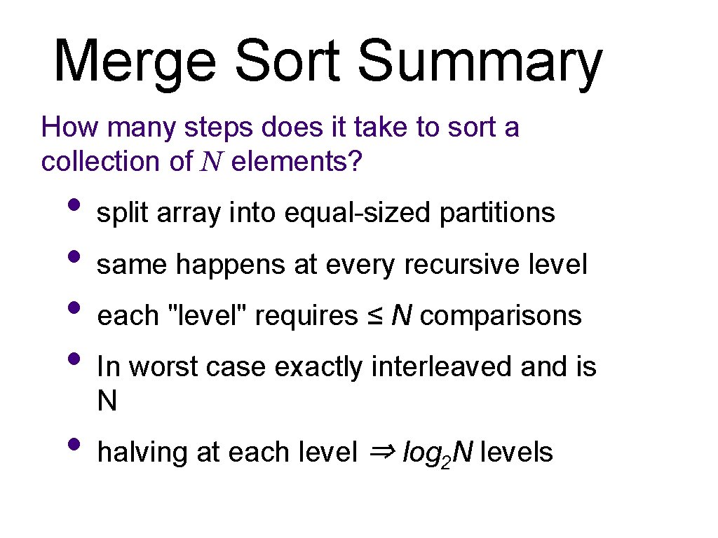
Merge Sort Summary How many steps does it take to sort a collection of N elements? • split array into equal-sized partitions • same happens at every recursive level • each "level" requires ≤ N comparisons • In worst case exactly interleaved and is N • halving at each level ⇒ log N levels 2

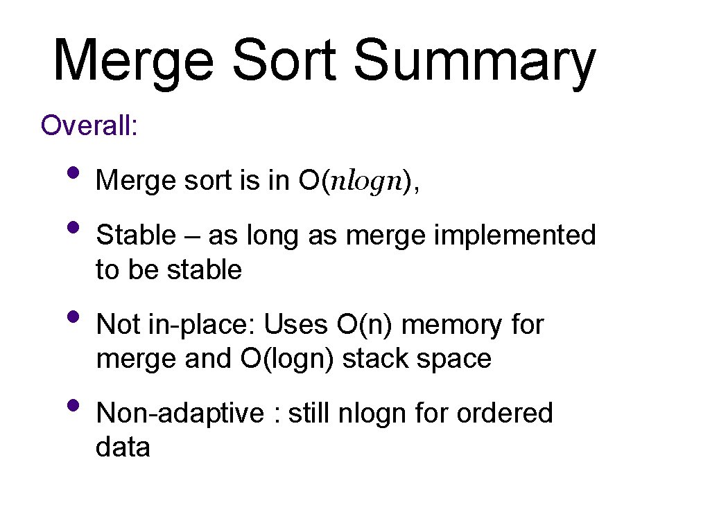
Merge Sort Summary Overall: • Merge sort is in O(nlogn), • Stable – as long as merge implemented to be stable • Not in-place: Uses O(n) memory for merge and O(logn) stack space • Non-adaptive : still nlogn for ordered data

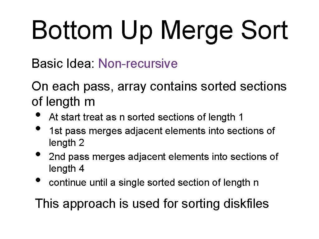
Bottom Up Merge Sort Basic Idea: Non-recursive On each pass, array contains sorted sections of length m • • At start treat as n sorted sections of length 1 1 st pass merges adjacent elements into sections of length 2 2 nd pass merges adjacent elements into sections of length 4 continue until a single sorted section of length n This approach is used for sorting diskfiles

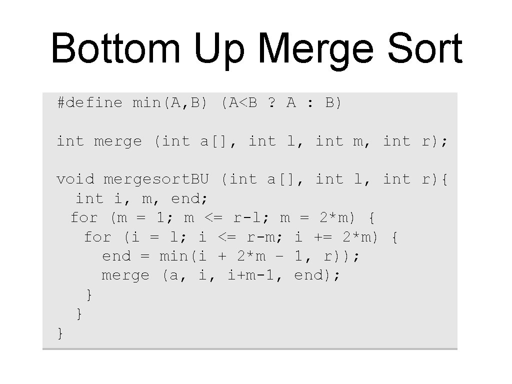
Bottom Up Merge Sort #define min(A, B) (A<B ? A : B) int merge (int a[], int l, int m, int r); void mergesort. BU (int a[], int l, int r){ int i, m, end; for (m = 1; m <= r-l; m = 2*m) { for (i = l; i <= r-m; i += 2*m) { end = min(i + 2*m – 1, r)); merge (a, i, i+m-1, end); } } }

Merge Sort on Lists Straight forward to implement on linked lists • Traverses its input in sequential order • Do not need extra space for merging lists • Works for top-down and bottom up versions

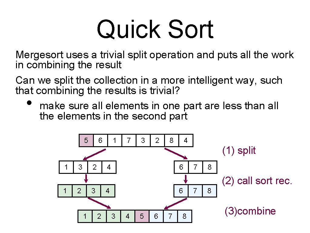
Quick Sort Mergesort uses a trivial split operation and puts all the work in combining the result Can we split the collection in a more intelligent way, such that combining the results is trivial? make sure all elements in one part are less than all the elements in the second part • 5 1 3 6 2 1 7 3 2 8 4 4 6 (1) split 7 8 (2) call sort rec. 1 2 3 1 4 2 6 3 4 5 6 7 8 (3)combine

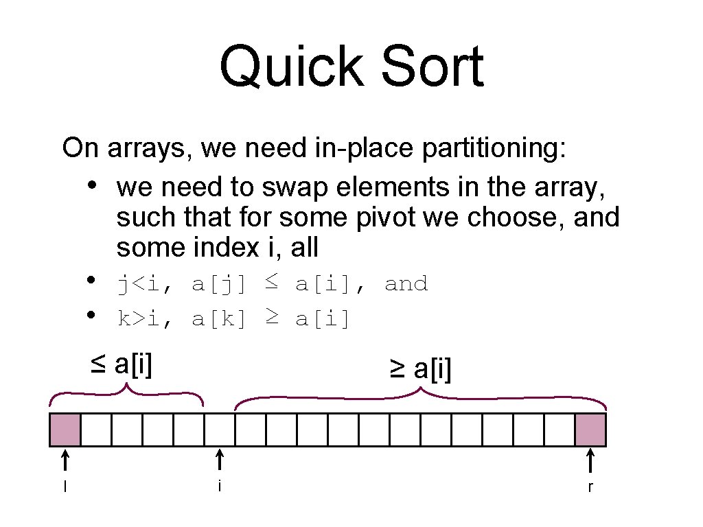
Quick Sort On arrays, we need in-place partitioning: • we need to swap elements in the array, such that for some pivot we choose, and some index i, all • j<i, a[j] ≤ a[i], and • k>i, a[k] ≥ a[i] ≤ a[i] l ≥ a[i] i r

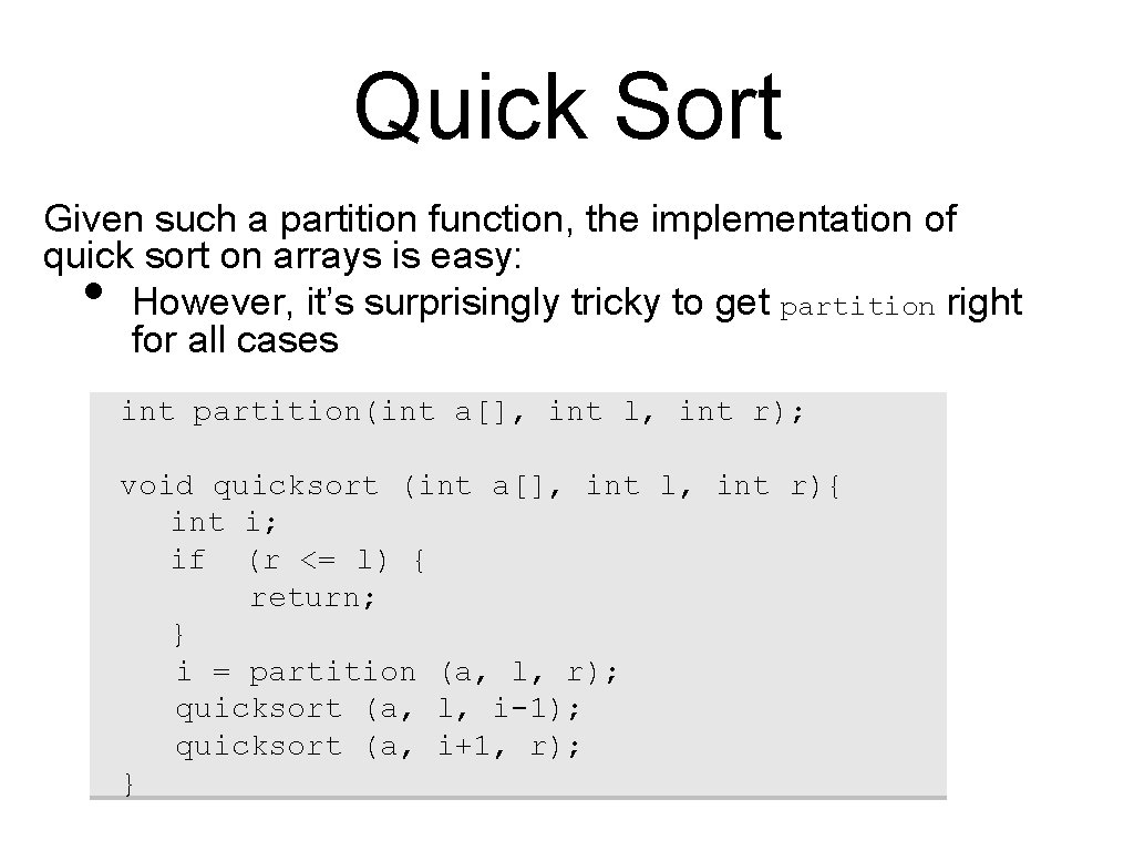
Quick Sort Given such a partition function, the implementation of quick sort on arrays is easy: However, it’s surprisingly tricky to get partition right for all cases • int partition(int a[], int l, int r); void quicksort (int a[], int l, int r){ int i; if (r <= l) { return; } i = partition (a, l, r); quicksort (a, l, i-1); quicksort (a, i+1, r); }

Quick Sort int partition (int a[], int l, int r) { int i = l-1; int j = r; int pivot = a[r]; //rightmost is pivot for (; ; ) { while ( a[++i] < pivot) ; while ( pivot < a[--j] && j != l); if (i >= j) { break; } swap(i, j, a); } //put pivot into place swap(i, r a); return i; //Index of the pivot }

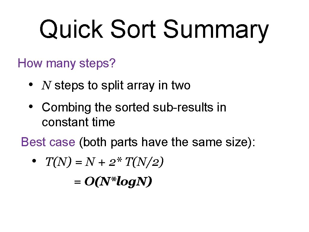
Quick Sort Summary How many steps? • N steps to split array in two • Combing the sorted sub-results in constant time Best case (both parts have the same size): • T(N) = N + 2* T(N/2) = O(N*log. N)

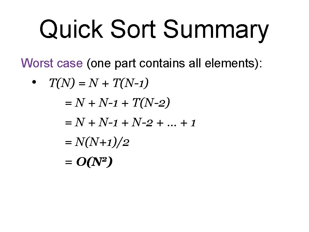
Quick Sort Summary Worst case (one part contains all elements): • T(N) = N + T(N-1) = N + N-1 + T(N-2) = N + N-1 + N-2 +. . . + 1 = N(N+1)/2 = 2 O(N )

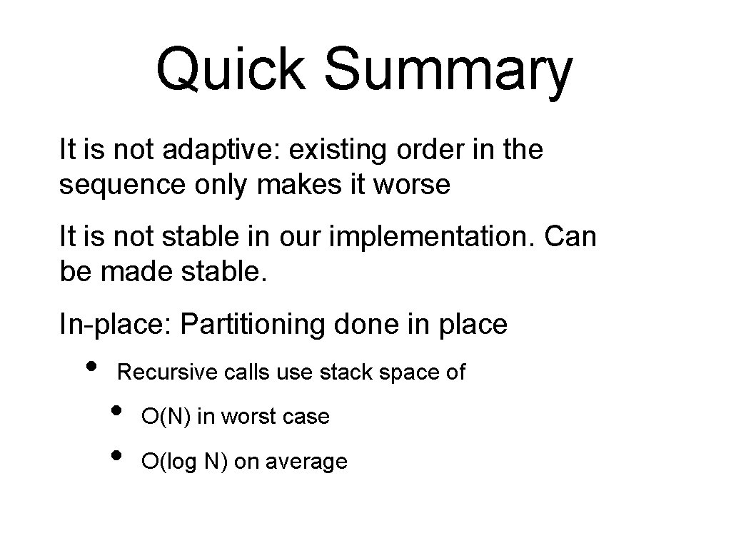
Quick Summary It is not adaptive: existing order in the sequence only makes it worse It is not stable in our implementation. Can be made stable. In-place: Partitioning done in place • Recursive calls use stack space of • • O(N) in worst case O(log N) on average

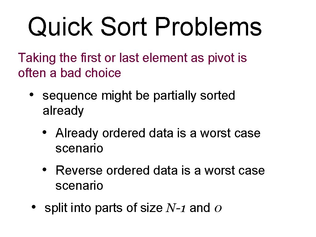
Quick Sort Problems Taking the first or last element as pivot is often a bad choice • sequence might be partially sorted already • Already ordered data is a worst case scenario • Reverse ordered data is a worst case scenario • split into parts of size N-1 and 0

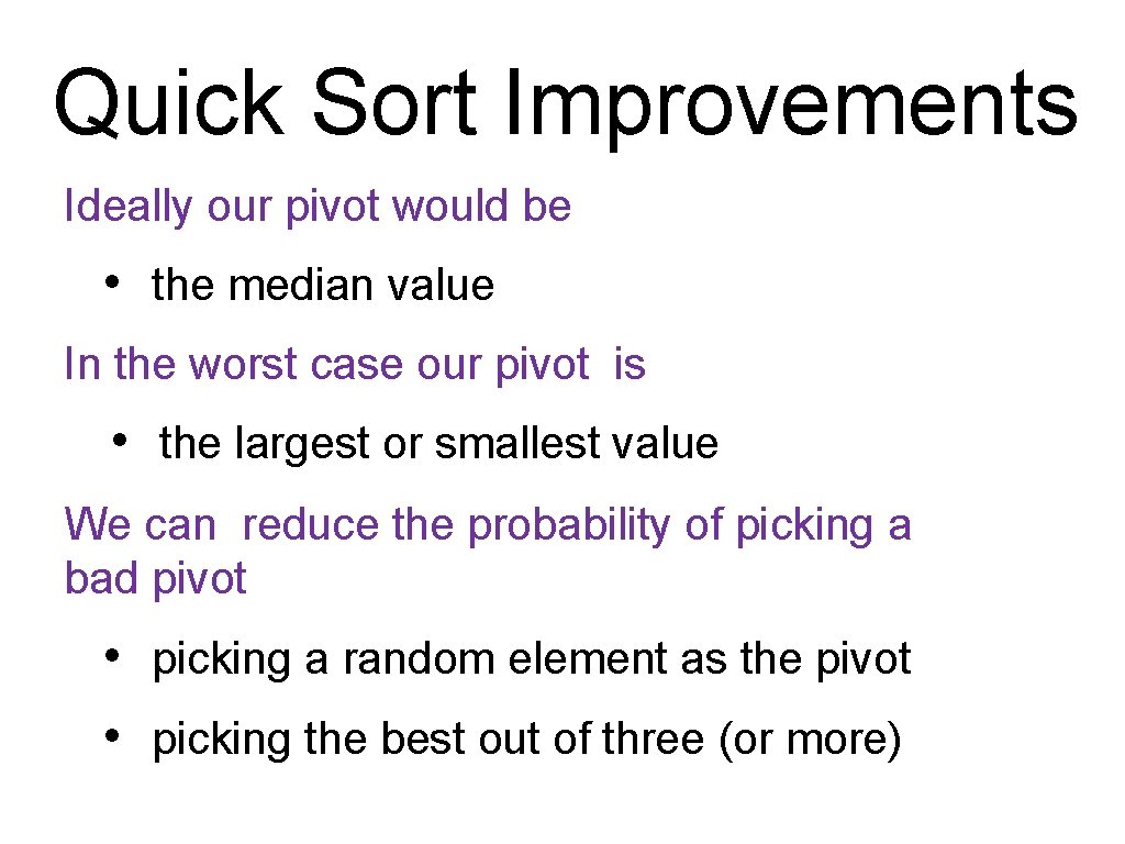
Quick Sort Improvements Ideally our pivot would be • the median value In the worst case our pivot is • the largest or smallest value We can reduce the probability of picking a bad pivot • picking a random element as the pivot • picking the best out of three (or more)

Quick Sort Improvements Median of Three Partitioning – choosing a better pivot • Compare left-most, middle and right-most element • Pick the median of these 3 values to be the pivot • Does not eliminate the worst case but makes it less likely • Ordered data no longer a worst case scenario

Median of Three Partitioning l (l+r)/2 (1) pick a[l], a[r], a[(r+l)/2] (2) swap a[r-1] and a[(r+l)/2] (3) sort a[l], a[r-1], a[r] such that a[l]<=a[r-1] <= a[r] (4) call partition on a[l+1] to a[r-1] r-1 r

Quick Sort Optimisation For small sequences, quick sort is relatively expensive because of the recursive calls • • Quick sort with subfile cutoff Handle small partitions less than a certain threshold length differently • • Switch to insertion sort for the small partitions Don’t sort. Leave and do insertion sort at the end Handling duplicates more efficiently by using three way partitioning.

Quicksort on Lists Straight forward to do if we just use first or last element as the pivot • Picking the pivot via randomisation or median of 3 is now O(n) instead of O(1).

Quick vs Merge Sort On typical modern architectures, efficient quicksort implementations generally outperform mergesort for sorting RAM-based arrays. • quick sort is also a cache friendly sorting algorithm as it has good locality of reference when used for arrays.

Quick vs Merge Sort On the other hand, merge sort is a stable sort, parallelizes better, and is more efficient at handling slow-to-access sequential media. Merge sort is often the best choice for sorting a linked list and the merging can be done without using extra space that is used during merge for arrays.

How fast can a sort become? All the sorts we have seen so far have been comparison based sorts • find order by comparing elements in the sequence • can sort any type of data as long as there is a way to compare 2 items

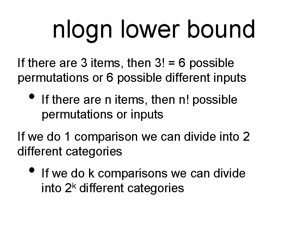
nlogn lower bound If there are 3 items, then 3! = 6 possible permutations or 6 possible different inputs • If there are n items, then n! possible permutations or inputs If we do 1 comparison we can divide into 2 different categories • If we do k comparisons we can divide into 2 k different categories

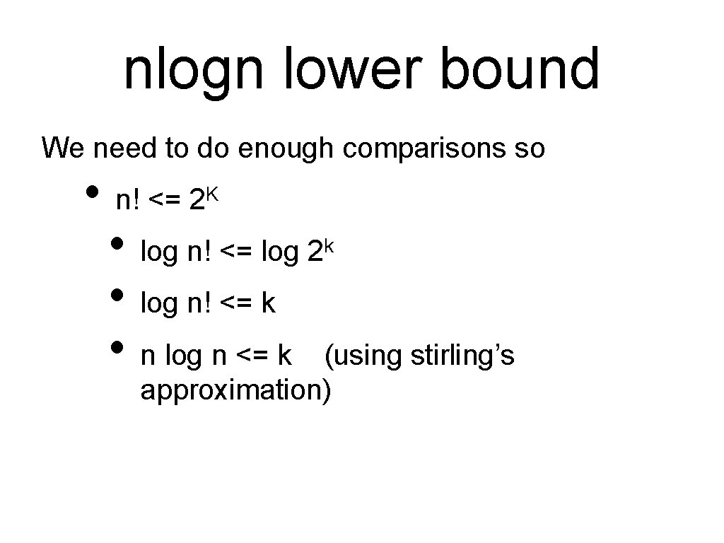
nlogn lower bound We need to do enough comparisons so • n! <= 2 • log n! <= log 2 • log n! <= k • n log n <= k (using stirling’s K k approximation)

How fast can a sort become? Theoretical lower bound on worst case running time of comparison based sorts is O(nlog(n)). • Algorithms such as quicksort and mergesort are really about as fast as we can go for unknown types of data.

Non-comparison Based Sorting We may not actually have to compare pairs of elements to sort the data. • Specialised sorts can be implemented if additional information about the data to be sorted is known. • Take advantage of special properties of keys • We can do some kinds of sorts in linear time!

Key Indexed Counting Sort Basic Idea: • Using an array, count up number of times each key appears • Use this information as an index of where the item belongs in the final sorted array • Place items in the final sorted array based on their index

Key Indexed Counting Sort For example: Sorting numbers from 0. . 10 • If I knew there were three 0’s and two 1’s • If I had a 2, it would go at index 5 • If I got another 2, it would go at index 6.

Key indexed Counting sort May work in O(n) time. How? • Because it uses no comparisons! • But we have to make assumptions about the size and nature of the data Assumptions • Sequence of size N • Each key is in the range of 0 - M-1

Key indexed Counting sort Time Complexity • Efficient if M is not too large compared to N • O(n + M) • Not good in cases like : 1, 2, 999999 • In-place? No. Uses temporary arrays of O(n+M) • Is stable

Radix Sorting Processing keys one piece at a time Keys are treated as numbers represented in base-R (radix) number system Binary numbers R is 2 Decimal numbers R is 10 Ascii strings R is 128 or 256 Unicode strings R is 65, 536 • • Sorting is done individually on each digit in the key one at a time – digit by digit or character by character

Radix Sort LSD Radix Sort Least Significant Digit First: • Consider characters or digits or bits from Right to Left (ie from least significant) • Stably sort using dth digit as the key • Can use Key Indexed Counting sort.

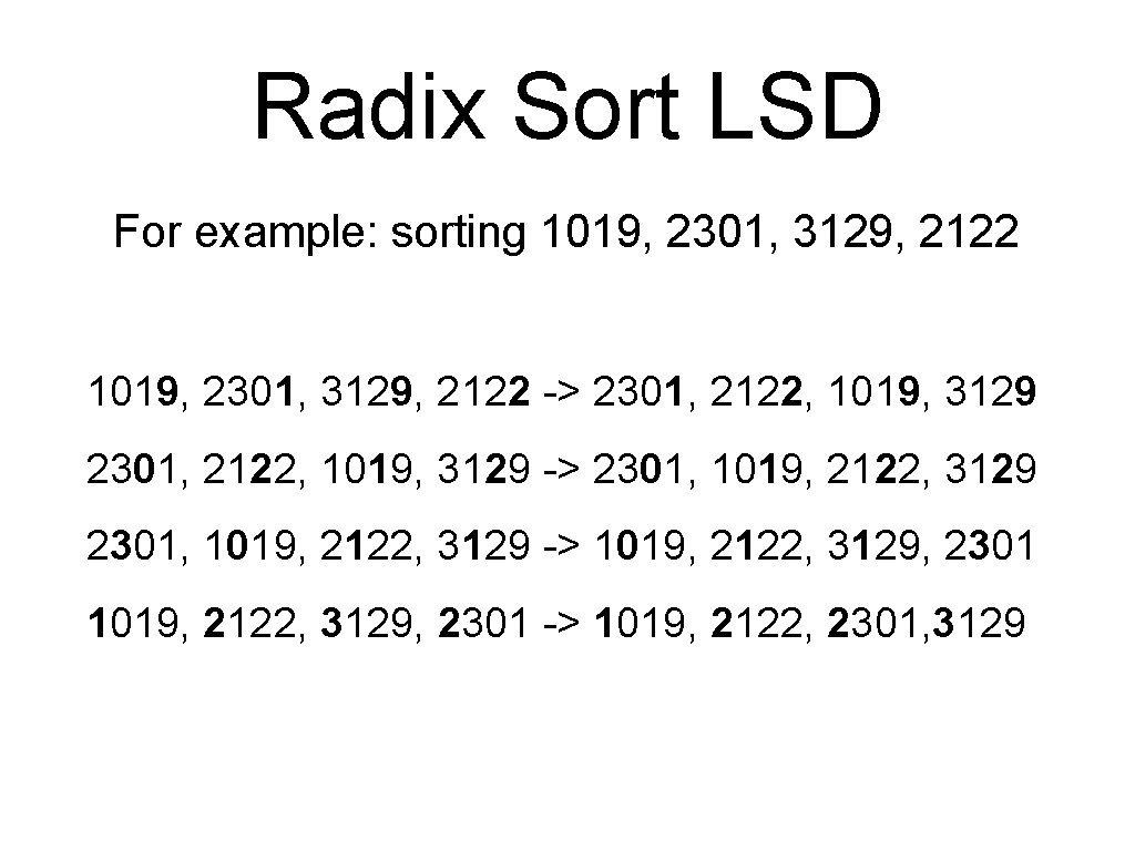
Radix Sort LSD For example: sorting 1019, 2301, 3129, 2122 -> 2301, 2122, 1019, 3129 -> 2301, 1019, 2122, 3129 -> 1019, 2122, 3129, 2301 -> 1019, 2122, 2301, 3129

Radix Sort LSD Summary Time complexity: O(w(n+R)) • w is the width of the data ie 987 is 3 digits wide, “aaa” is 3 characters, integers (binary rep) could have w as 32 and R of 2 • The algorithm makes w passes over all n keys.

Radix Sort LSD Summary Not in place: extra space: O(n + R) Stable Can modify to use for variable length data Imagine sorting strings like • “zaaaaaaa” and “aaaa” • Can spend lots of work comparing insignificant details

Radix Sort MSD Radix Sort Most Significant Digit First: • Partition file into R pieces according to first character • Can use key-indexed counting • Recursively sort all strings that start with each character • key-indexed counts delineate files to sort

Radix Sort MSD Summary Time complexity: O(w(n+R)) Extra space O(N + DR) D is depth of recursion) Stability depends on implementation Don't have to go through all of the digits to get a sorted array. This can make MSD radix sort considerably faster Can use insertion sort for small subfiles