Distributed Visual Model Learning for Large Scale Object

Distributed Visual Model Learning for Large Scale Object Recognition Speaker: A/Prof. Liang Lin jointly work with Xiaolong Wang, Xiaodan Liang, Zechao Yang, et al. Lab of Intelligent Media Computing, Sun Yat-Sen University

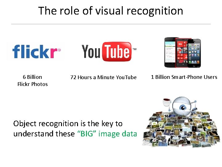
The role of visual recognition 6 Billion Flickr Photos 72 Hours a Minute You. Tube Object recognition is the key to understand these “BIG” image data 1 Billion Smart-Phone Users

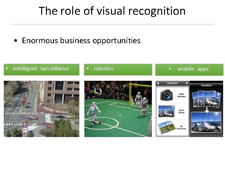
The role of visual recognition • Enormous business opportunities • intelligent surveillance • robotics • mobile apps

Outline of this talk • Background and motivation • Compositional (part-based) object model • Learning object model in distributed systems

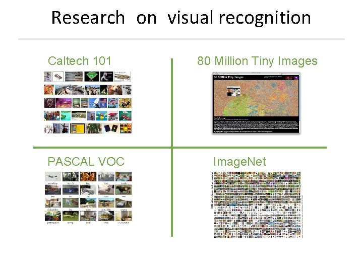
Research on visual recognition Caltech 101 PASCAL VOC 80 Million Tiny Images Image. Net

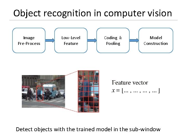
Object recognition in computer vision Image Pre-Process Low-Level Feature Coding & Pooling Model Construction Detect objects with the trained model in the sub-window

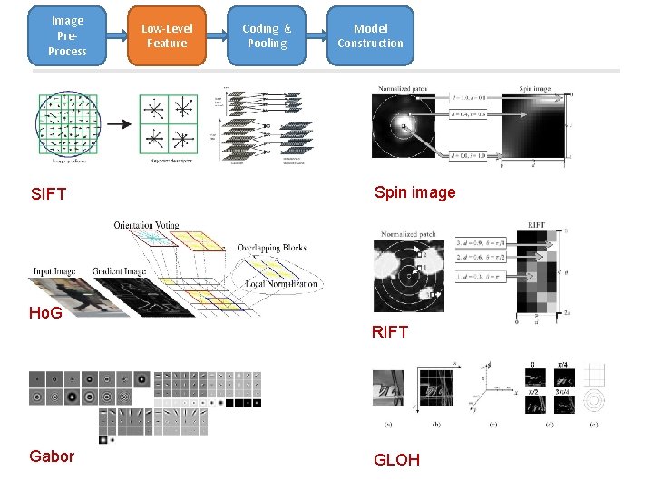
Image Pre. Process SIFT Low-Level Feature Coding & Pooling Model Construction Spin image Ho. G RIFT Gabor GLOH

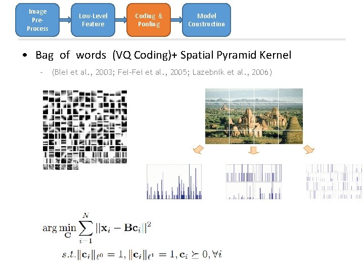
Image Pre. Process Low-Level Feature Coding & Pooling Model Construction • Bag of words (VQ Coding)+ Spatial Pyramid Kernel – (Blei et al. , 2003; Fei-Fei et al. , 2005; Lazebnik et al. , 2006)

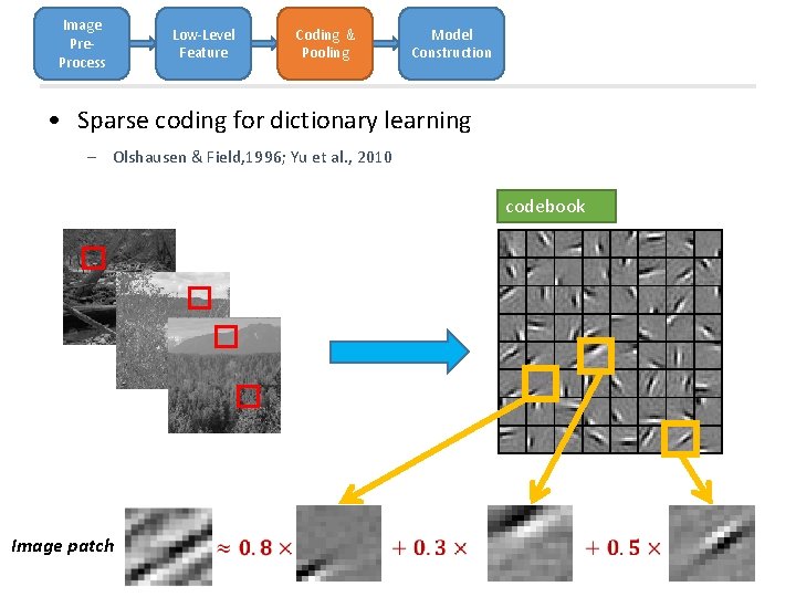
Image Pre. Process Low-Level Feature Coding & Pooling Model Construction • Sparse coding for dictionary learning – Olshausen & Field, 1996; Yu et al. , 2010 codebook Image patch

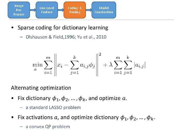
Image Pre. Process • Low-Level Feature Coding & Pooling Model Construction

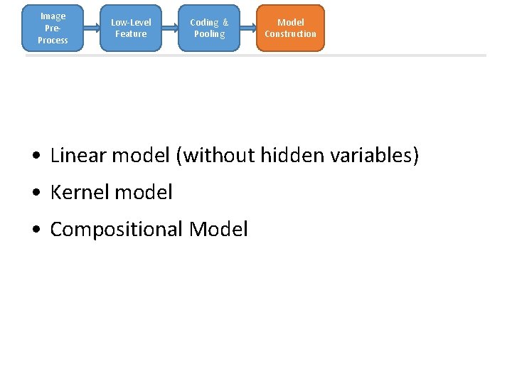
Image Pre. Process Low-Level Feature Coding & Pooling Model Construction • Linear model (without hidden variables) • Kernel model • Compositional Model

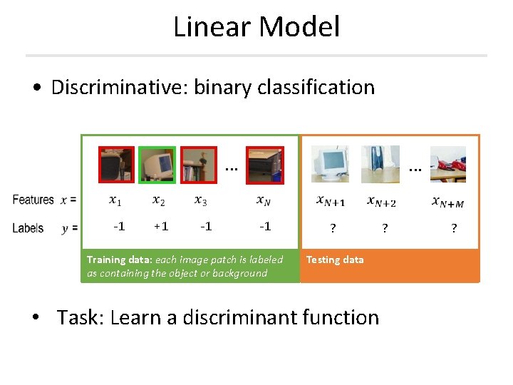
Linear Model • Discriminative: binary classification … -1 +1 … -1 Training data: each image patch is labeled as containing the object or background ? Testing data • Task: Learn a discriminant function ? ?

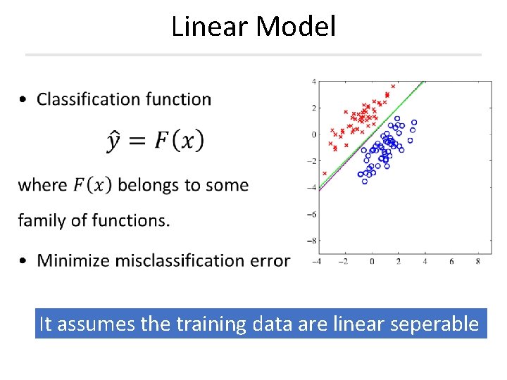
Linear Model It assumes the training data are linear seperable

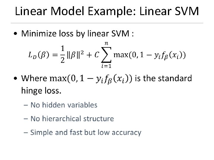
Linear Model Example: Linear SVM •

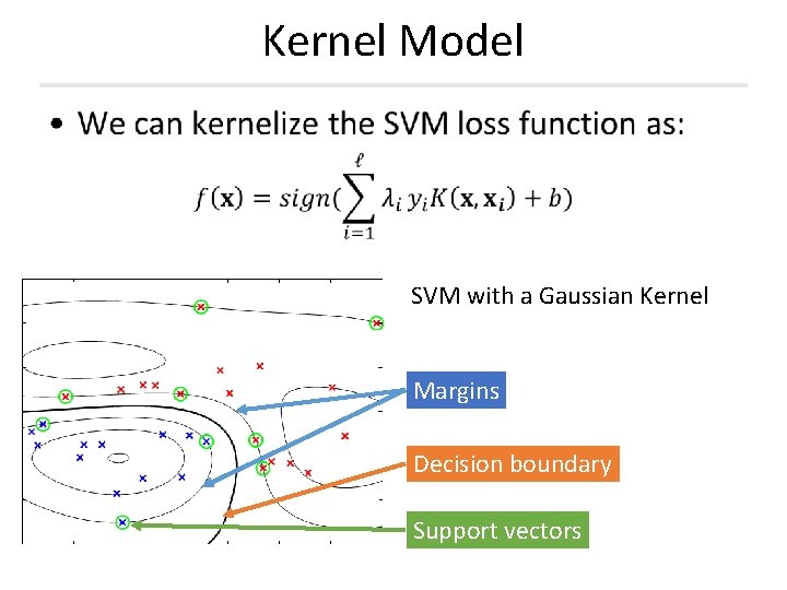
Kernel Model • SVM with a Gaussian Kernel Margins Decision boundary Support vectors

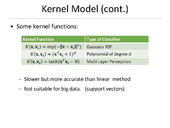
Kernel Model (cont. ) • Some kernel functions: Kernel Function Type of Classifier Gaussian RBF Multi Layer Perceptron – Slower but more accurate than linear method – Not suitable for big data. (support vectors)

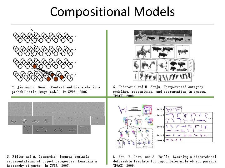
Compositional Models Y. Jin and S. Geman. Context and hierarchy in a probabilistic image model. In CVPR, 2006. S. Fidler and A. Leonardis. Towards scalable representations of object categories: Learning a hierarchy of parts. In CVPR, 2007. S. Todorovic and N. Ahuja. Unsupervised category modeling, recognition, and segmentation in images. TPAMI, 2008. L. Zhu, Y. Chen, and A. Yuille. Learning a hierarchical deformable template for rapid deformable object parsing. TPAMI, 2009.

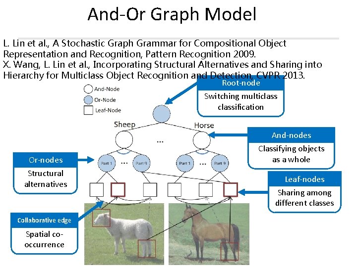
And-Or Graph Model L. Lin et al. , A Stochastic Graph Grammar for Compositional Object Representation and Recognition, Pattern Recognition 2009. X. Wang, L. Lin et al. , Incorporating Structural Alternatives and Sharing into Hierarchy for Multiclass Object Recognition and Detection, CVPR 2013. Root-node Switching multiclassification Or-nodes Structural alternatives Collaborative edge Spatial cooccurrence And-nodes Classifying objects as a whole Leaf-nodes Sharing among different classes

Outline of this talk • Background and motivation • Compositional (part-based) object model • Learning object model in distributed systems

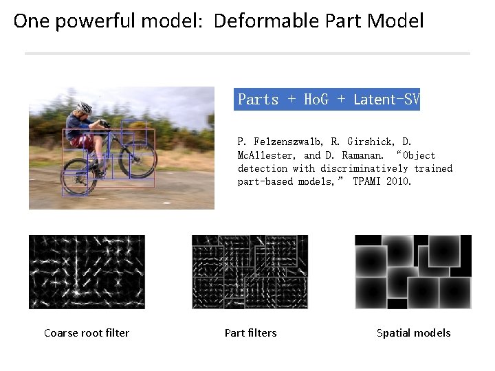
One powerful model: Deformable Part Model Parts + Ho. G + Latent-SVM P. Felzenszwalb, R. Girshick, D. Mc. Allester, and D. Ramanan. “Object detection with discriminatively trained part-based models, ” TPAMI 2010. Coarse root filter Part filters Spatial models

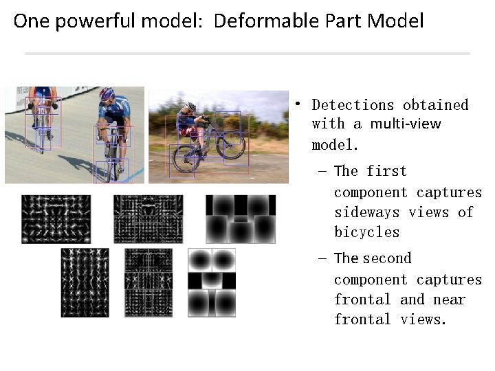
One powerful model: Deformable Part Model • Detections obtained with a multi-view model. – The first component captures sideways views of bicycles – The second component captures frontal and near frontal views.

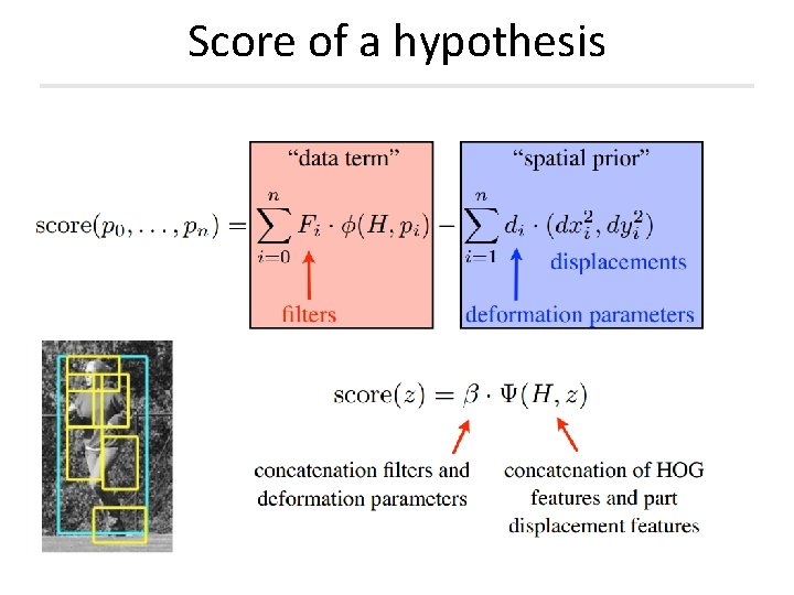
Score of a hypothesis

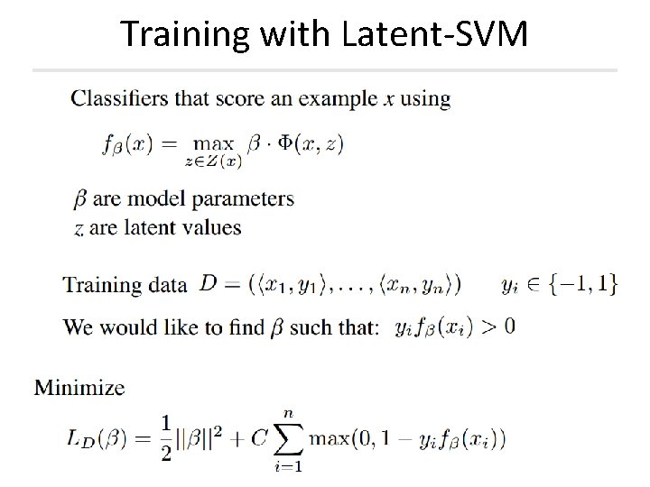
Training with Latent-SVM

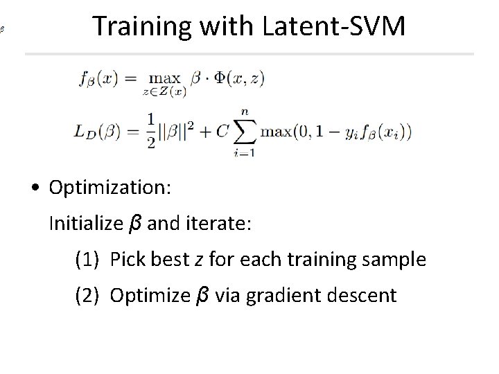
Training with Latent-SVM • Optimization: Initialize β and iterate: (1) Pick best z for each training sample (2) Optimize β via gradient descent

Outline of this talk • Background and motivation • Compositional (part-based) object model • Learning object model in distributed systems

Learning in distributed systems • Taking training on PASCAL VOC 2007 as an example (including around 10000 training samples and 20 object classes). • We use 100 computers to train 20 models. The data are distributed in these computers and each of them stores 100 training image.

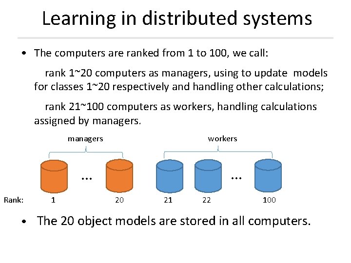
Learning in distributed systems • The computers are ranked from 1 to 100, we call: rank 1~20 computers as managers, using to update models for classes 1~20 respectively and handling other calculations; rank 21~100 computers as workers, handling calculations assigned by managers workers … … Rank: 1 20 21 22 100 • The 20 object models are stored in all computers.

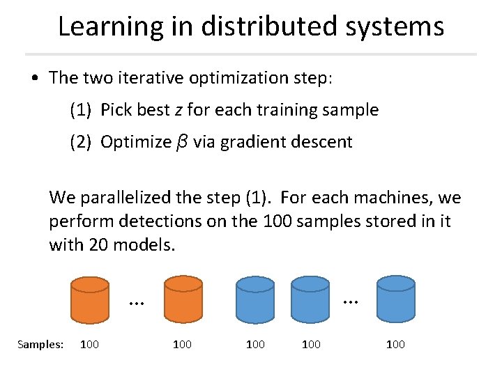
Learning in distributed systems • The two iterative optimization step: (1) Pick best z for each training sample (2) Optimize β via gradient descent We parallelized the step (1). For each machines, we perform detections on the 100 samples stored in it with 20 models. … … Samples: 100 100 100

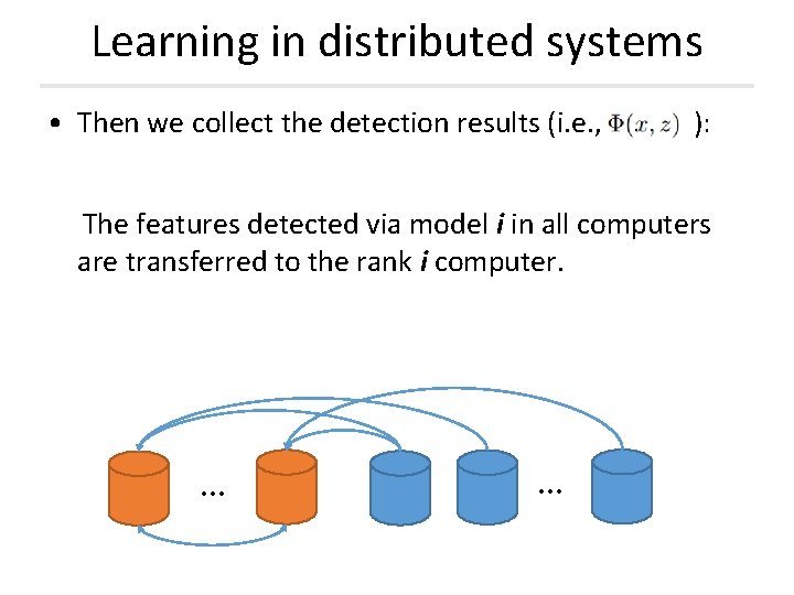
Learning in distributed systems • Then we collect the detection results (i. e. , ): The features detected via model i in all computers are transferred to the rank i computer. … …

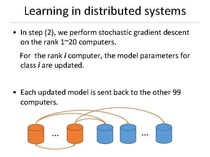
Learning in distributed systems • In step (2), we perform stochastic gradient descent on the rank 1~20 computers. For the rank i computer, the model parameters for class i are updated. • Each updated model is sent back to the other 99 computers. … …

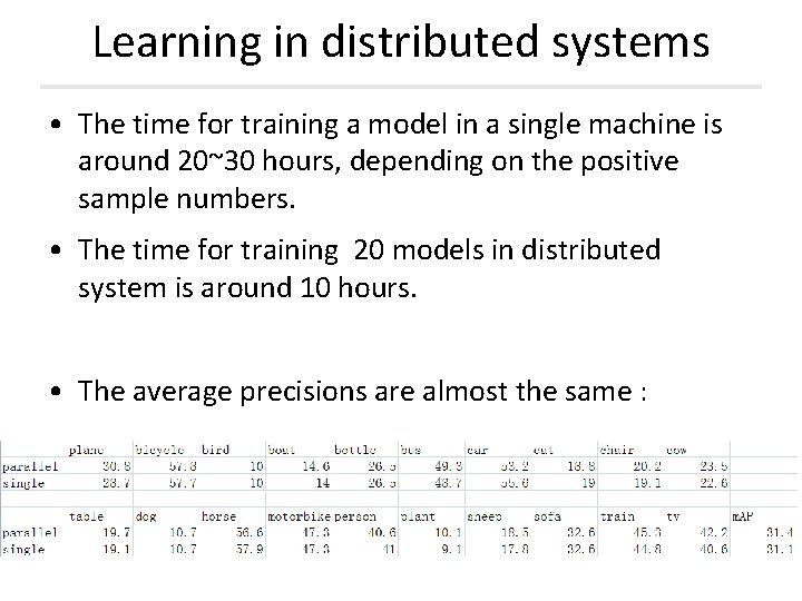
Learning in distributed systems • The time for training a model in a single machine is around 20~30 hours, depending on the positive sample numbers. • The time for training 20 models in distributed system is around 10 hours. • The average precisions are almost the same :

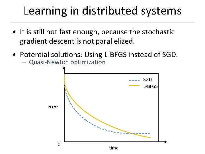
Learning in distributed systems • It is still not fast enough, because the stochastic gradient descent is not parallelized. • Potential solutions: Using L-BFGS instead of SGD. – Quasi-Newton optimization SGD L-BFGS error 0 time

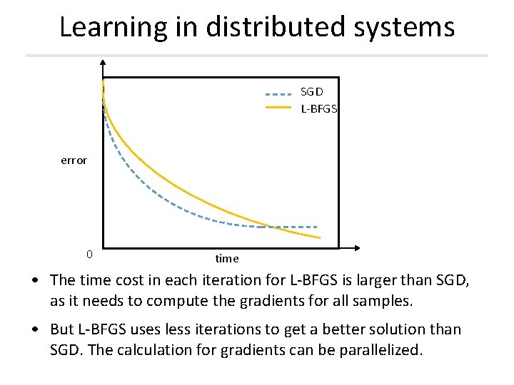
Learning in distributed systems SGD L-BFGS error 0 time • The time cost in each iteration for L-BFGS is larger than SGD, as it needs to compute the gradients for all samples. • But L-BFGS uses less iterations to get a better solution than SGD. The calculation for gradients can be parallelized.

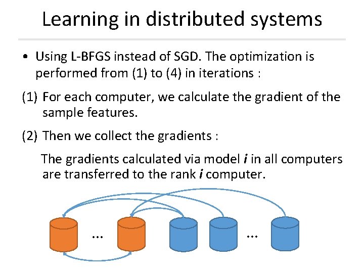
Learning in distributed systems • Using L-BFGS instead of SGD. The optimization is performed from (1) to (4) in iterations : (1) For each computer, we calculate the gradient of the sample features. (2) Then we collect the gradients : The gradients calculated via model i in all computers are transferred to the rank i computer. … …

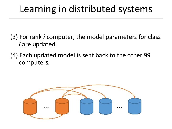
Learning in distributed systems (3) For rank i computer, the model parameters for class i are updated. (4) Each updated model is sent back to the other 99 computers. … …

Learning in distributed systems • The experiments are still on pending, because of the CVPR 2014 deadline – We are expecting the proportional improvement on efficiency – e. g. approximately 100 times faster on a distributed system of 100 workstations

Q&A Thank You! MORE INFORMATION: HTTP: //VISION. SYSU. EDU. CN