Distributed Memory Machines and Programming Lecture 7 James

Distributed Memory Machines and Programming Lecture 7 James Demmel www. cs. berkeley. edu/~demmel/cs 267_Spr 13 Slides from Kathy Yelick CS 267 Lecture 7 1

Recap of Lecture 6 • Shared memory multiprocessors • Caches may be either shared or distributed. • Multicore chips are likely to have shared caches • Cache hit performance is better if they are distributed (each cache is smaller/closer) but they must be kept coherent -- multiple cached copies of same location must be kept equal. • Requires clever hardware (see CS 258, CS 252). • Distant memory much more expensive to access. • Machines scale to 10 s or 100 s of processors. • Shared memory programming • Starting, stopping threads. • Communication by reading/writing shared variables. • Synchronization with locks, barriers. 02/12/2013 CS 267 Lecture 7 2

Outline • Distributed Memory Architectures • Properties of communication networks • Topologies • Performance models • Programming Distributed Memory Machines using Message Passing • Overview of MPI • Basic send/receive use • Non-blocking communication • Collectives 02/12/2013 CS 267 Lecture 7 3

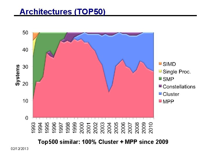
Architectures (TOP 50) Top 500 similar: 100% Cluster + MPP since 2009 02/12/2013

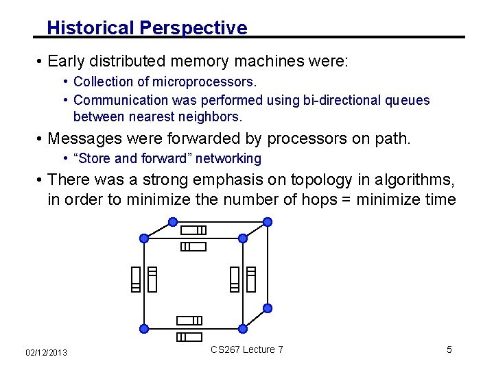
Historical Perspective • Early distributed memory machines were: • Collection of microprocessors. • Communication was performed using bi-directional queues between nearest neighbors. • Messages were forwarded by processors on path. • “Store and forward” networking • There was a strong emphasis on topology in algorithms, in order to minimize the number of hops = minimize time 02/12/2013 CS 267 Lecture 7 5

Network Analogy • To have a large number of different transfers occurring at once, you need a large number of distinct wires • Not just a bus, as in shared memory • Networks are like streets: • • Link = street. Switch = intersection. Distances (hops) = number of blocks traveled. Routing algorithm = travel plan. • Properties: • Latency: how long to get between nodes in the network. • Street: time for one car = dist (miles) / speed (miles/hr) • Bandwidth: how much data can be moved per unit time. • Street: cars/hour = density (cars/mile) * speed (miles/hr) * #lanes • Network bandwidth is limited by the bit rate per wire and #wires 02/12/2013 CS 267 Lecture 7 6

Design Characteristics of a Network • Topology (how things are connected) • Crossbar; ring; 2 -D, 3 -D, higher-D mesh or torus; hypercube; tree; butterfly; perfect shuffle. . • Routing algorithm: • Example in 2 D torus: all east-west then all north -south (avoids deadlock). • Switching strategy: • Circuit switching: full path reserved for entire message, like the telephone. • Packet switching: message broken into separatelyrouted packets, like the post office, or internet • Flow control (what if there is congestion): • Stall, store data temporarily in buffers, re-route data to other nodes, tell source node to temporarily halt, discard, etc. 02/12/2013 CS 267 Lecture 7 7

Performance Properties of a Network: Latency • Diameter: the maximum (over all pairs of nodes) of the shortest path between a given pair of nodes. • Latency: delay between send and receive times • Latency tends to vary widely across architectures • Vendors often report hardware latencies (wire time) • Application programmers care about software latencies (user program to user program) • Observations: • Latencies differ by 1 -2 orders across network designs • Software/hardware overhead at source/destination dominate cost (1 s-10 s usecs) • Hardware latency varies with distance (10 s-100 s nsec per hop) but is small compared to overheads • Latency is key for programs with many small messages 02/12/2013 CS 267 Lecture 7 8

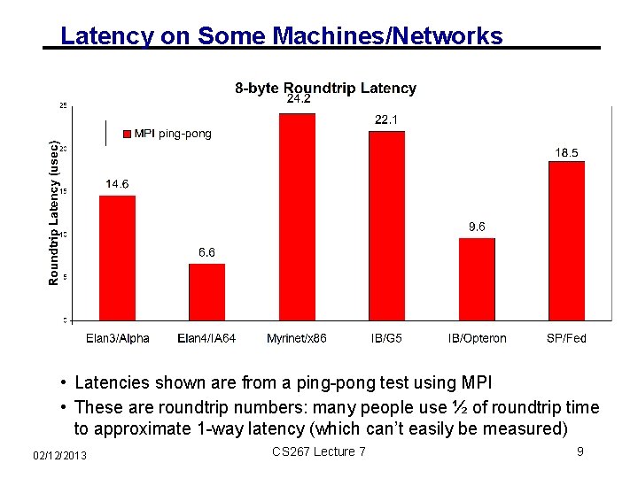
Latency on Some Machines/Networks • Latencies shown are from a ping-pong test using MPI • These are roundtrip numbers: many people use ½ of roundtrip time to approximate 1 -way latency (which can’t easily be measured) 02/12/2013 CS 267 Lecture 7 9

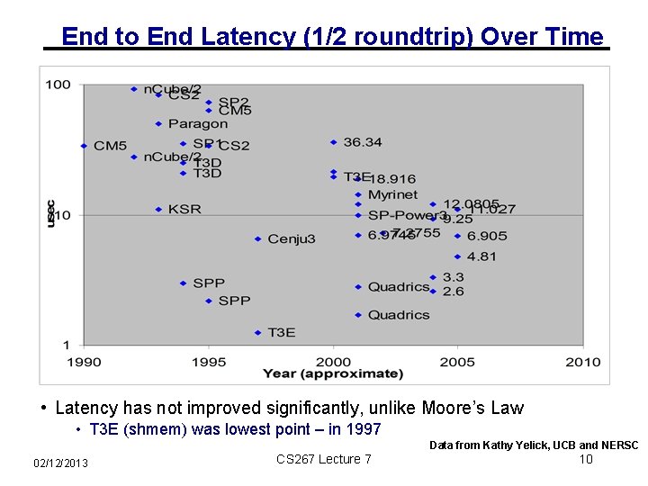
End to End Latency (1/2 roundtrip) Over Time • Latency has not improved significantly, unlike Moore’s Law • T 3 E (shmem) was lowest point – in 1997 Data from Kathy Yelick, UCB and NERSC 02/12/2013 CS 267 Lecture 7 10

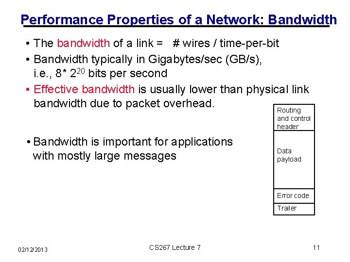
Performance Properties of a Network: Bandwidth • The bandwidth of a link = # wires / time-per-bit • Bandwidth typically in Gigabytes/sec (GB/s), i. e. , 8* 220 bits per second • Effective bandwidth is usually lower than physical link bandwidth due to packet overhead. Routing and control header • Bandwidth is important for applications with mostly large messages Data payload Error code Trailer 02/12/2013 CS 267 Lecture 7 11

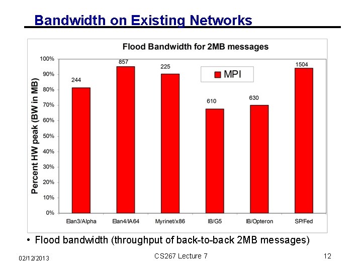
Bandwidth on Existing Networks • Flood bandwidth (throughput of back-to-back 2 MB messages) 02/12/2013 CS 267 Lecture 7 12

Bandwidth Chart Note: bandwidth depends on SW, not just HW Data from Mike Welcome, NERSC 02/12/2013 CS 267 Lecture 7 13

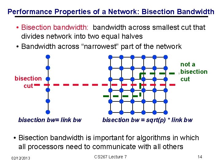
Performance Properties of a Network: Bisection Bandwidth • Bisection bandwidth: bandwidth across smallest cut that divides network into two equal halves • Bandwidth across “narrowest” part of the network not a bisection cut bisection bw= link bw bisection bw = sqrt(p) * link bw • Bisection bandwidth is important for algorithms in which all processors need to communicate with all others 02/12/2013 CS 267 Lecture 7 14

Network Topology • In the past, there was considerable research in network topology and in mapping algorithms to topology. • Key cost to be minimized: number of “hops” between nodes (e. g. “store and forward”) • Modern networks hide hop cost (i. e. , “wormhole routing”), so topology less of a factor in performance of many algorithms • Example: On IBM SP system, hardware latency varies from 0. 5 usec to 1. 5 usec, but user-level message passing latency is roughly 36 usec. • Need some background in network topology • Algorithms may have a communication topology • Example later of big performance impact 02/12/2013 CS 267 Lecture 7 15

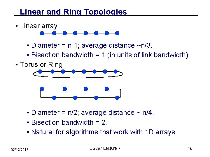
Linear and Ring Topologies • Linear array • Diameter = n-1; average distance ~n/3. • Bisection bandwidth = 1 (in units of link bandwidth). • Torus or Ring • Diameter = n/2; average distance ~ n/4. • Bisection bandwidth = 2. • Natural for algorithms that work with 1 D arrays. 02/12/2013 CS 267 Lecture 7 16

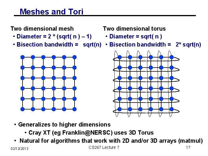
Meshes and Tori Two dimensional mesh Two dimensional torus • Diameter = 2 * (sqrt( n ) – 1) • Diameter = sqrt( n ) • Bisection bandwidth = sqrt(n) • Bisection bandwidth = 2* sqrt(n) • Generalizes to higher dimensions • Cray XT (eg Franklin@NERSC) uses 3 D Torus • Natural for algorithms that work with 2 D and/or 3 D arrays (matmul) 02/12/2013 CS 267 Lecture 7 17

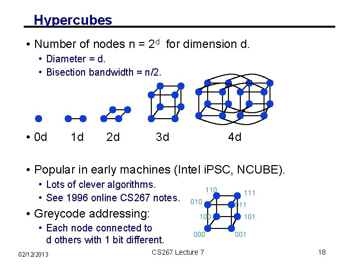
Hypercubes • Number of nodes n = 2 d for dimension d. • Diameter = d. • Bisection bandwidth = n/2. • 0 d 1 d 2 d 3 d 4 d • Popular in early machines (Intel i. PSC, NCUBE). • Lots of clever algorithms. • See 1996 online CS 267 notes. • Greycode addressing: 010 100 • Each node connected to d others with 1 bit different. 02/12/2013 110 000 CS 267 Lecture 7 111 011 101 001 18

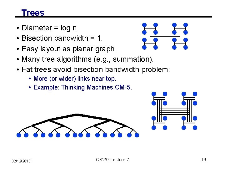
Trees • • • Diameter = log n. Bisection bandwidth = 1. Easy layout as planar graph. Many tree algorithms (e. g. , summation). Fat trees avoid bisection bandwidth problem: • More (or wider) links near top. • Example: Thinking Machines CM-5. 02/12/2013 CS 267 Lecture 7 19

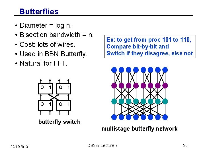
Butterflies • • • Diameter = log n. Bisection bandwidth = n. Cost: lots of wires. Used in BBN Butterfly. Natural for FFT. O 1 O 1 Ex: to get from proc 101 to 110, Compare bit-by-bit and Switch if they disagree, else not butterfly switch multistage butterfly network 02/12/2013 CS 267 Lecture 7 20

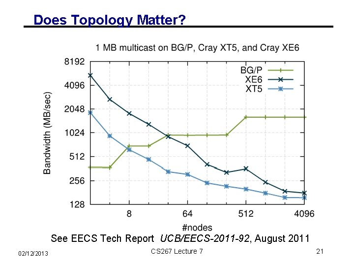
Does Topology Matter? See EECS Tech Report UCB/EECS-2011 -92, August 2011 02/12/2013 CS 267 Lecture 7 21

Evolution of Distributed Memory Machines • Special queue connections are being replaced by direct memory access (DMA): • Processor packs or copies messages. • Initiates transfer, goes on computing. • Wormhole routing in hardware: • Special message processors do not interrupt main processors along path. • Long message sends are pipelined. • Processors don’t wait for complete message before forwarding • Message passing libraries provide store-and-forward abstraction: • Can send/receive between any pair of nodes, not just along one wire. • Time depends on distance since each processor along path must participate. 02/12/2013 CS 267 Lecture 7 23

Performance Models CS 267 Lecture 7 24

Shared Memory Performance Models • Parallel Random Access Memory (PRAM) • All memory access operations complete in one clock period -- no concept of memory hierarchy (“too good to be true”). • OK for understanding whether an algorithm has enough parallelism at all (see CS 273). • Parallel algorithm design strategy: first do a PRAM algorithm, then worry about memory/communication time (sometimes works) • Slightly more realistic versions exist • E. g. , Concurrent Read Exclusive Write (CREW) PRAM. • Still missing the memory hierarchy 02/12/2013 CS 267 Lecture 7 25

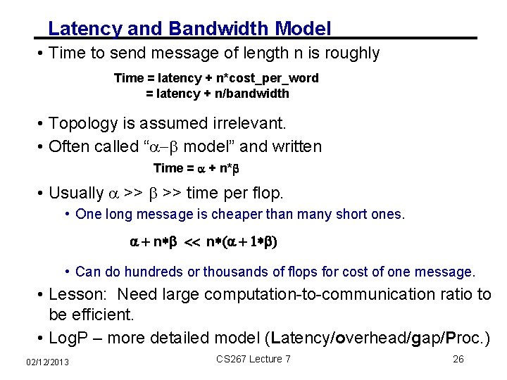
Latency and Bandwidth Model • Time to send message of length n is roughly Time = latency + n*cost_per_word = latency + n/bandwidth • Topology is assumed irrelevant. • Often called “a-b model” and written Time = a + n*b • Usually a >> b >> time per flop. • One long message is cheaper than many short ones. a + n*b << n*(a + 1*b) • Can do hundreds or thousands of flops for cost of one message. • Lesson: Need large computation-to-communication ratio to be efficient. • Log. P – more detailed model (Latency/overhead/gap/Proc. ) 02/12/2013 CS 267 Lecture 7 26

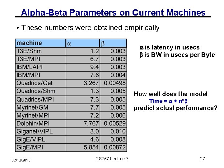
Alpha-Beta Parameters on Current Machines • These numbers were obtained empirically a is latency in usecs b is BW in usecs per Byte How well does the model Time = a + n*b predict actual performance? 02/12/2013 CS 267 Lecture 7 27

Model Time Varying Message Size & Machines 02/12/2013 CS 267 Lecture 7 28

Measured Message Time 02/12/2013 CS 267 Lecture 7 29

Programming Distributed Memory Machines with Message Passing Slides from Jonathan Carter (jtcarter@lbl. gov), Katherine Yelick (yelick@cs. berkeley. edu), Bill Gropp (wgropp@illinois. edu) 02/12/2013 CS 267 Lecture 7 35

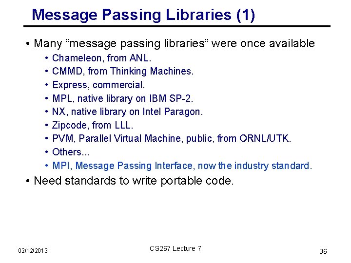
Message Passing Libraries (1) • Many “message passing libraries” were once available • • • Chameleon, from ANL. CMMD, from Thinking Machines. Express, commercial. MPL, native library on IBM SP-2. NX, native library on Intel Paragon. Zipcode, from LLL. PVM, Parallel Virtual Machine, public, from ORNL/UTK. Others. . . MPI, Message Passing Interface, now the industry standard. • Need standards to write portable code. 02/12/2013 CS 267 Lecture 7 36

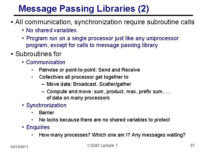
Message Passing Libraries (2) • All communication, synchronization require subroutine calls • No shared variables • Program run on a single processor just like any uniprocessor program, except for calls to message passing library • Subroutines for • Communication • • Pairwise or point-to-point: Send and Receive Collectives all processor get together to – Move data: Broadcast, Scatter/gather – Compute and move: sum, product, max, prefix sum, … of data on many processors • Synchronization • • Barrier No locks because there are no shared variables to protect • Enquiries • 02/12/2013 How many processes? Which one am I? Any messages waiting? CS 267 Lecture 7 37

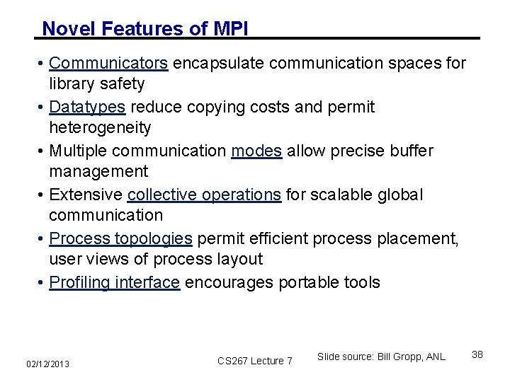
Novel Features of MPI • Communicators encapsulate communication spaces for library safety • Datatypes reduce copying costs and permit heterogeneity • Multiple communication modes allow precise buffer management • Extensive collective operations for scalable global communication • Process topologies permit efficient process placement, user views of process layout • Profiling interface encourages portable tools 02/12/2013 CS 267 Lecture 7 Slide source: Bill Gropp, ANL 38

MPI References • The Standard itself: • at http: //www. mpi-forum. org • All MPI official releases, in both postscript and HTML • Other information on Web: • at http: //www. mcs. anl. gov/mpi • pointers to lots of stuff, including other talks and tutorials, a FAQ, other MPI pages 02/12/2013 CS 267 Lecture 7 Slide source: Bill Gropp, ANL 39

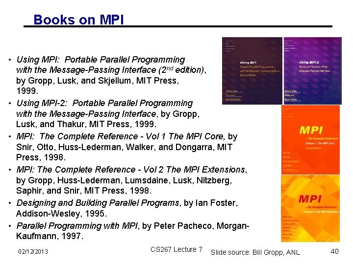
Books on MPI • Using MPI: Portable Parallel Programming with the Message-Passing Interface (2 nd edition), by Gropp, Lusk, and Skjellum, MIT Press, 1999. • Using MPI-2: Portable Parallel Programming with the Message-Passing Interface, by Gropp, Lusk, and Thakur, MIT Press, 1999. • MPI: The Complete Reference - Vol 1 The MPI Core, by Snir, Otto, Huss-Lederman, Walker, and Dongarra, MIT Press, 1998. • MPI: The Complete Reference - Vol 2 The MPI Extensions, by Gropp, Huss-Lederman, Lumsdaine, Lusk, Nitzberg, Saphir, and Snir, MIT Press, 1998. • Designing and Building Parallel Programs, by Ian Foster, Addison-Wesley, 1995. • Parallel Programming with MPI, by Peter Pacheco, Morgan. Kaufmann, 1997. 02/12/2013 CS 267 Lecture 7 Slide source: Bill Gropp, ANL 40

Finding Out About the Environment • Two important questions that arise early in a parallel program are: • How many processes are participating in this computation? • Which one am I? • MPI provides functions to answer these questions: • MPI_Comm_size reports the number of processes. • MPI_Comm_rank reports the rank, a number between 0 and size-1, identifying the calling process 02/12/2013 CS 267 Lecture 7 Slide source: Bill Gropp, ANL 42

Hello (C) #include "mpi. h" #include <stdio. h> int main( int argc, char *argv[] ) { int rank, size; MPI_Init( &argc, &argv ); MPI_Comm_rank( MPI_COMM_WORLD, &rank ); MPI_Comm_size( MPI_COMM_WORLD, &size ); printf( "I am %d of %dn", rank, size ); MPI_Finalize(); return 0; } Note: hidden slides show Fortran and C++ versions of each example 02/12/2013 CS 267 Lecture 7 Slide source: Bill Gropp, ANL 43

Notes on Hello World • All MPI programs begin with MPI_Init and end with MPI_Finalize • MPI_COMM_WORLD is defined by mpi. h (in C) or mpif. h (in Fortran) and designates all processes in the MPI “job” • Each statement executes independently in each process • including the printf/print statements • I/O not part of MPI-1 but is in MPI-2 • print and write to standard output or error not part of either MPI 1 or MPI-2 • output order is undefined (may be interleaved by character, line, or blocks of characters), • The MPI-1 Standard does not specify how to run an MPI program, but many implementations provide mpirun –np 4 a. out 02/12/2013 CS 267 Lecture 7 Slide source: Bill Gropp, ANL 46

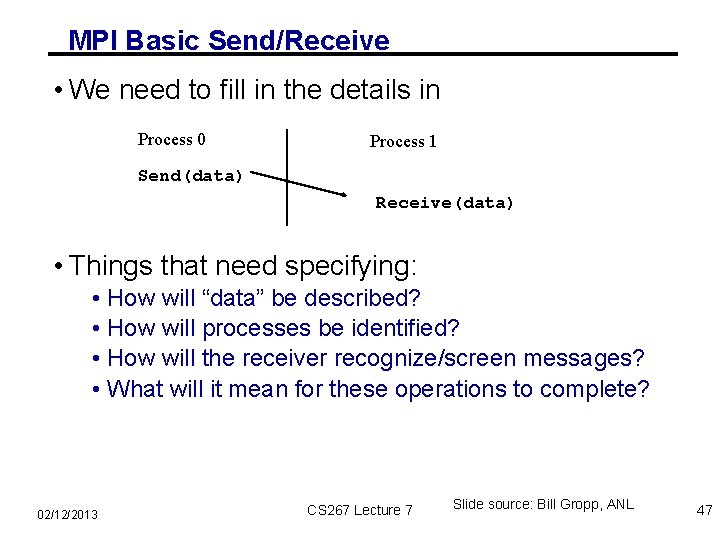
MPI Basic Send/Receive • We need to fill in the details in Process 0 Process 1 Send(data) Receive(data) • Things that need specifying: • How will “data” be described? • How will processes be identified? • How will the receiver recognize/screen messages? • What will it mean for these operations to complete? 02/12/2013 CS 267 Lecture 7 Slide source: Bill Gropp, ANL 47

Some Basic Concepts • Processes can be collected into groups • Each message is sent in a context, and must be received in the same context • Provides necessary support for libraries • A group and context together form a communicator • A process is identified by its rank in the group associated with a communicator • There is a default communicator whose group contains all initial processes, called MPI_COMM_WORLD 02/12/2013 CS 267 Lecture 7 Slide source: Bill Gropp, ANL 48

MPI Datatypes • The data in a message to send or receive is described by a triple (address, count, datatype), where • An MPI datatype is recursively defined as: • predefined, corresponding to a data type from the language (e. g. , MPI_INT, MPI_DOUBLE) • a contiguous array of MPI datatypes • a strided block of datatypes • an indexed array of blocks of datatypes • an arbitrary structure of datatypes • There are MPI functions to construct custom datatypes, in particular ones for subarrays • May hurt performance if datatypes are complex 02/12/2013 CS 267 Lecture 7 Slide source: Bill Gropp, ANL 49

MPI Tags • Messages are sent with an accompanying userdefined integer tag, to assist the receiving process in identifying the message • Messages can be screened at the receiving end by specifying a specific tag, or not screened by specifying MPI_ANY_TAG as the tag in a receive • Some non-MPI message-passing systems have called tags “message types”. MPI calls them tags to avoid confusion with datatypes 02/12/2013 CS 267 Lecture 7 Slide source: Bill Gropp, ANL 50

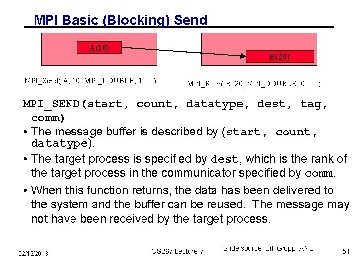
MPI Basic (Blocking) Send A(10) B(20) MPI_Send( A, 10, MPI_DOUBLE, 1, …) MPI_Recv( B, 20, MPI_DOUBLE, 0, … ) MPI_SEND(start, count, datatype, dest, tag, comm) • The message buffer is described by (start, count, datatype). • The target process is specified by dest, which is the rank of the target process in the communicator specified by comm. • When this function returns, the data has been delivered to the system and the buffer can be reused. The message may not have been received by the target process. 02/12/2013 CS 267 Lecture 7 Slide source: Bill Gropp, ANL 51

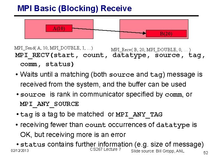
MPI Basic (Blocking) Receive A(10) B(20) MPI_Send( A, 10, MPI_DOUBLE, 1, …) MPI_Recv( B, 20, MPI_DOUBLE, 0, … ) MPI_RECV(start, count, datatype, source, tag, comm, status) • Waits until a matching (both source and tag) message is received from the system, and the buffer can be used • source is rank in communicator specified by comm, or MPI_ANY_SOURCE • tag is a tag to be matched or MPI_ANY_TAG • receiving fewer than count occurrences of datatype is OK, but receiving more is an error • status contains further information (e. g. size of message) 02/12/2013 CS 267 Lecture 7 Slide source: Bill Gropp, ANL 52

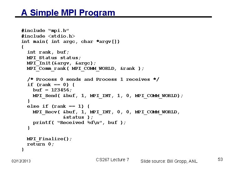
A Simple MPI Program #include “mpi. h” #include <stdio. h> int main( int argc, char *argv[]) { int rank, buf; MPI_Status status; MPI_Init(&argv, &argc); MPI_Comm_rank( MPI_COMM_WORLD, &rank ); /* Process 0 sends and Process 1 receives */ if (rank == 0) { buf = 123456; MPI_Send( &buf, 1, MPI_INT, 1, 0, MPI_COMM_WORLD); } else if (rank == 1) { MPI_Recv( &buf, 1, MPI_INT, 0, 0, MPI_COMM_WORLD, &status ); printf( “Received %dn”, buf ); } } MPI_Finalize(); return 0; 02/12/2013 CS 267 Lecture 7 Slide source: Bill Gropp, ANL 53

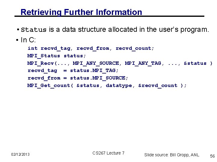
Retrieving Further Information • Status is a data structure allocated in the user’s program. • In C: int recvd_tag, recvd_from, recvd_count; MPI_Status status; MPI_Recv(. . . , MPI_ANY_SOURCE, MPI_ANY_TAG, . . . , &status ) recvd_tag = status. MPI_TAG; recvd_from = status. MPI_SOURCE; MPI_Get_count( &status, datatype, &recvd_count ); 02/12/2013 CS 267 Lecture 7 Slide source: Bill Gropp, ANL 56

Tags and Contexts • Separation of messages used to be accomplished by use of tags, but • this requires libraries to be aware of tags used by other libraries. • this can be defeated by use of “wild card” tags. • Contexts are different from tags • no wild cards allowed • allocated dynamically by the system when a library sets up a communicator for its own use. • User-defined tags still provided in MPI for user convenience in organizing application 02/12/2013 CS 267 Lecture 7 Slide source: Bill Gropp, ANL 58

MPI is Simple • Many parallel programs can be written using just these six functions, only two of which are non-trivial: • MPI_INIT • MPI_FINALIZE • MPI_COMM_SIZE • MPI_COMM_RANK • MPI_SEND • MPI_RECV 02/12/2013 CS 267 Lecture 7 Slide source: Bill Gropp, ANL 60

Another Approach to Parallelism • Collective routines provide a higher-level way to organize a parallel program • Each process executes the same communication operations • MPI provides a rich set of collective operations… 02/12/2013 CS 267 Lecture 7 Slide source: Bill Gropp, ANL 61

Collective Operations in MPI • Collective operations are called by all processes in a communicator • MPI_BCAST distributes data from one process (the root) to all others in a communicator • MPI_REDUCE combines data from all processes in communicator and returns it to one process • In many numerical algorithms, SEND/RECEIVE can be replaced by BCAST/REDUCE, improving both simplicity and efficiency 02/12/2013 CS 267 Lecture 7 Slide source: Bill Gropp, ANL 62

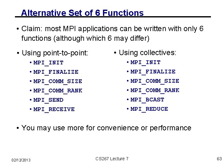
Alternative Set of 6 Functions • Claim: most MPI applications can be written with only 6 functions (although which 6 may differ) • Using point-to-point: • MPI_INIT • MPI_FINALIZE • MPI_COMM_SIZE • MPI_COMM_RANK • MPI_SEND • MPI_RECEIVE • Using collectives: • MPI_INIT • MPI_FINALIZE • MPI_COMM_SIZE • MPI_COMM_RANK • MPI_BCAST • MPI_REDUCE • You may use more for convenience or performance 02/12/2013 CS 267 Lecture 7 63

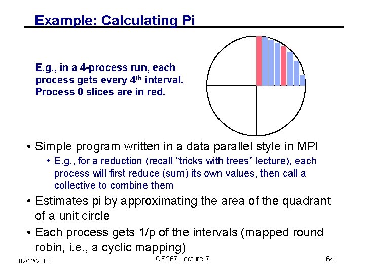
Example: Calculating Pi E. g. , in a 4 -process run, each process gets every 4 th interval. Process 0 slices are in red. • Simple program written in a data parallel style in MPI • E. g. , for a reduction (recall “tricks with trees” lecture), each process will first reduce (sum) its own values, then call a collective to combine them • Estimates pi by approximating the area of the quadrant of a unit circle • Each process gets 1/p of the intervals (mapped round robin, i. e. , a cyclic mapping) 02/12/2013 CS 267 Lecture 7 64

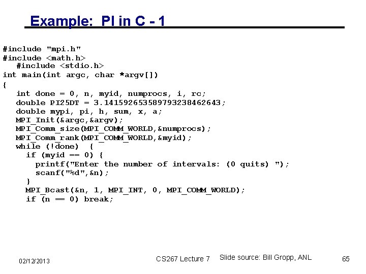
Example: PI in C - 1 #include "mpi. h" #include <math. h> #include <stdio. h> int main(int argc, char *argv[]) { int done = 0, n, myid, numprocs, i, rc; double PI 25 DT = 3. 141592653589793238462643; double mypi, h, sum, x, a; MPI_Init(&argc, &argv); MPI_Comm_size(MPI_COMM_WORLD, &numprocs); MPI_Comm_rank(MPI_COMM_WORLD, &myid); while (!done) { if (myid == 0) { printf("Enter the number of intervals: (0 quits) "); scanf("%d", &n); } MPI_Bcast(&n, 1, MPI_INT, 0, MPI_COMM_WORLD); if (n == 0) break; 02/12/2013 CS 267 Lecture 7 Slide source: Bill Gropp, ANL 65

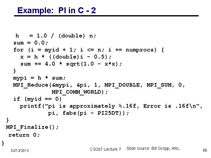
Example: PI in C - 2 h = 1. 0 / (double) n; sum = 0. 0; for (i = myid + 1; i <= n; i += numprocs) { x = h * ((double)i - 0. 5); sum += 4. 0 * sqrt(1. 0 - x*x); } mypi = h * sum; MPI_Reduce(&mypi, &pi, 1, MPI_DOUBLE, MPI_SUM, 0, MPI_COMM_WORLD); if (myid == 0) printf("pi is approximately %. 16 f, Error is. 16 fn", pi, fabs(pi - PI 25 DT)); } MPI_Finalize(); return 0; } 02/12/2013 CS 267 Lecture 7 Slide source: Bill Gropp, ANL 66

Synchronization • MPI_Barrier( comm ) • Blocks until all processes in the group of the communicator comm call it. • Almost never required in a parallel program • Occasionally useful in measuring performance and load balancing 02/12/2013 CS 267 Lecture 7 72

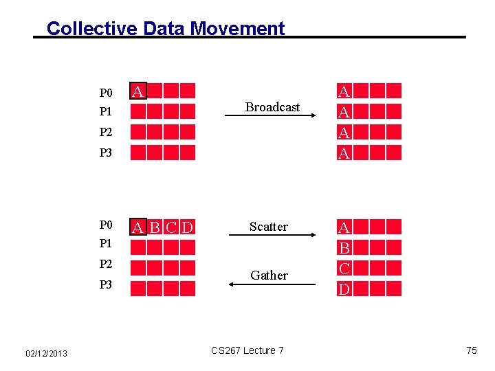
Collective Data Movement P 0 A P 1 Broadcast P 2 P 3 P 0 ABCD Scatter P 1 P 2 P 3 02/12/2013 Gather CS 267 Lecture 7 A A A B C D 75

Comments on Broadcast • All collective operations must be called by all processes in the communicator • MPI_Bcast is called by both the sender (called the root process) and the processes that are to receive the broadcast • MPI_Bcast is not a “multi-send” • “root” argument is the rank of the sender; this tells MPI which process originates the broadcast and which receive 02/12/2013 CS 267 Lecture 7 76

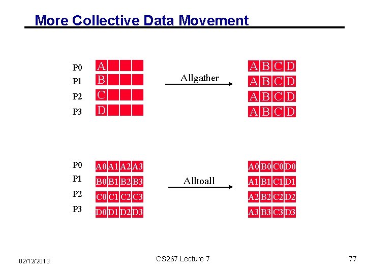
More Collective Data Movement P 3 A B C D P 0 A 1 A 2 A 3 P 1 B 0 B 1 B 2 B 3 P 2 C 0 C 1 C 2 C 3 A 2 B 2 C 2 D 2 P 3 D 0 D 1 D 2 D 3 A 3 B 3 C 3 D 3 P 0 P 1 P 2 02/12/2013 Allgather A A B B C C D D A 0 B 0 C 0 D 0 Alltoall CS 267 Lecture 7 A 1 B 1 C 1 D 1 77

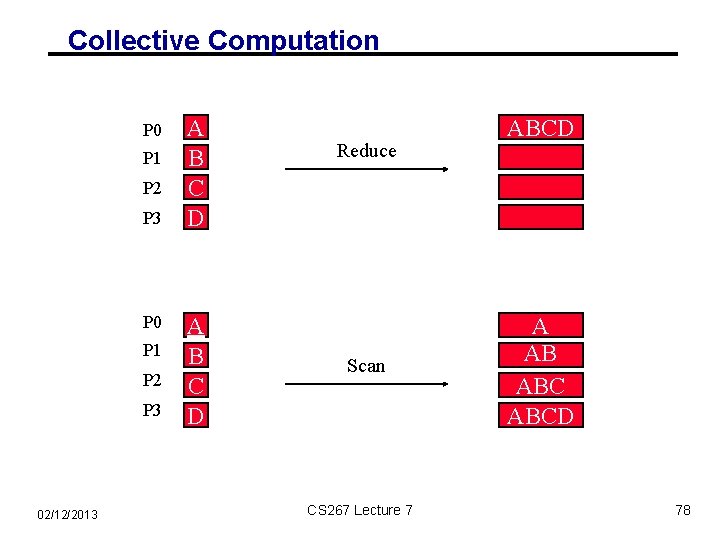
Collective Computation P 0 P 1 P 2 P 3 02/12/2013 A B C D Reduce Scan CS 267 Lecture 7 ABCD A AB ABCD 78

MPI Collective Routines • Many Routines: Allgather, Allgatherv, Allreduce, Alltoallv, Bcast, Gatherv, Reduce_scatter, Scan, Scatterv • All versions deliver results to all participating processes. • V versions allow the hunks to have variable sizes. • Allreduce, Reduce_scatter, and Scan take both built-in and user-defined combiner functions. • MPI-2 adds Alltoallw, Exscan, intercommunicator versions of most routines 02/12/2013 CS 267 Lecture 7 79

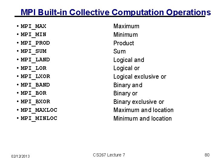
MPI Built-in Collective Computation Operations • MPI_MAX • MPI_MIN • MPI_PROD • MPI_SUM • MPI_LAND • MPI_LOR • MPI_LXOR • MPI_BAND • MPI_BOR • MPI_BXOR • MPI_MAXLOC • MPI_MINLOC 02/12/2013 Maximum Minimum Product Sum Logical and Logical or Logical exclusive or Binary and Binary or Binary exclusive or Maximum and location Minimum and location CS 267 Lecture 7 80

More on Message Passing • Message passing is a simple programming model, but there are some special issues • Buffering and deadlock • Deterministic execution • Performance 02/12/2013 CS 267 Lecture 7 Slide source: Bill Gropp, ANL 81

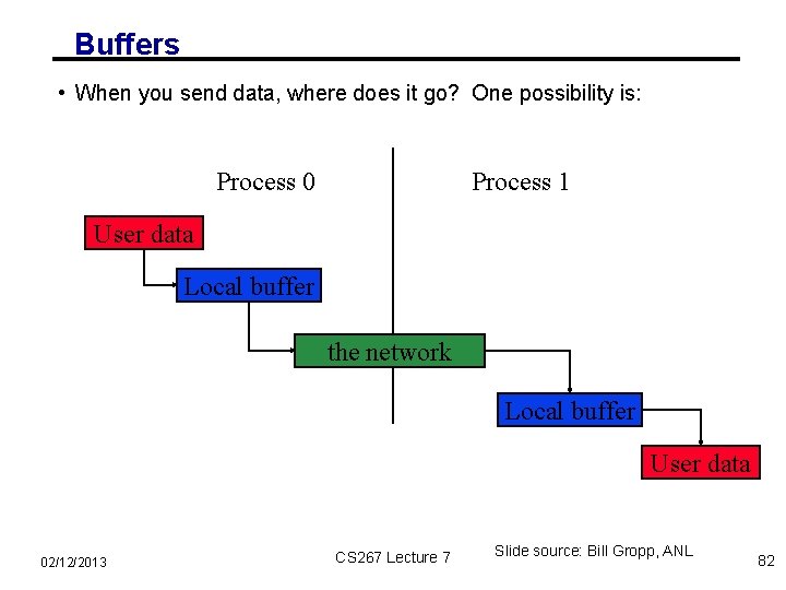
Buffers • When you send data, where does it go? One possibility is: Process 0 Process 1 User data Local buffer the network Local buffer User data 02/12/2013 CS 267 Lecture 7 Slide source: Bill Gropp, ANL 82

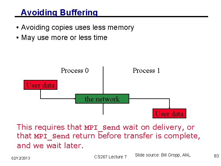
Avoiding Buffering • Avoiding copies uses less memory • May use more or less time Process 0 Process 1 User data the network User data This requires that MPI_Send wait on delivery, or that MPI_Send return before transfer is complete, and we wait later. 02/12/2013 CS 267 Lecture 7 Slide source: Bill Gropp, ANL 83

Blocking and Non-blocking Communication • So far we have been using blocking communication: • MPI_Recv does not complete until the buffer is full (available for use). • MPI_Send does not complete until the buffer is empty (available for use). • Completion depends on size of message and amount of system buffering. 02/12/2013 CS 267 Lecture 7 Slide source: Bill Gropp, ANL 84

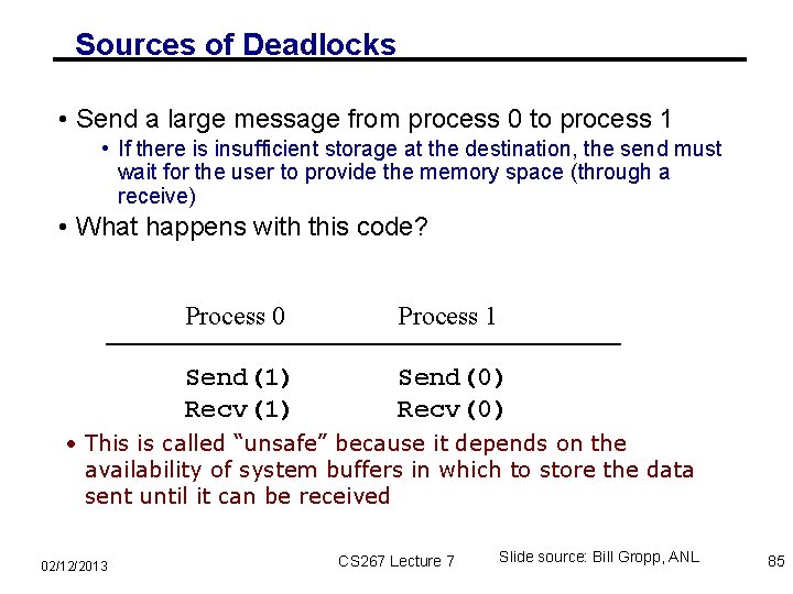
Sources of Deadlocks • Send a large message from process 0 to process 1 • If there is insufficient storage at the destination, the send must wait for the user to provide the memory space (through a receive) • What happens with this code? Process 0 Process 1 Send(1) Recv(1) Send(0) Recv(0) • This is called “unsafe” because it depends on the availability of system buffers in which to store the data sent until it can be received 02/12/2013 CS 267 Lecture 7 Slide source: Bill Gropp, ANL 85

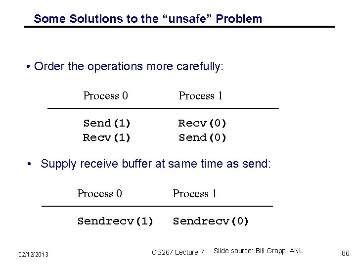
Some Solutions to the “unsafe” Problem • Order the operations more carefully: Process 0 Process 1 Send(1) Recv(0) Send(0) • Supply receive buffer at same time as send: 02/12/2013 Process 0 Process 1 Sendrecv(1) Sendrecv(0) CS 267 Lecture 7 Slide source: Bill Gropp, ANL 86

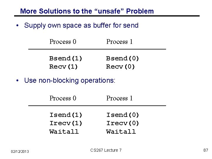
More Solutions to the “unsafe” Problem • Supply own space as buffer for send Process 0 Process 1 Bsend(1) Recv(1) Bsend(0) Recv(0) • Use non-blocking operations: 02/12/2013 Process 0 Process 1 Isend(1) Irecv(1) Waitall Isend(0) Irecv(0) Waitall CS 267 Lecture 7 87

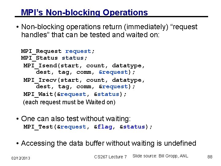
MPI’s Non-blocking Operations • Non-blocking operations return (immediately) “request handles” that can be tested and waited on: MPI_Request request; MPI_Status status; MPI_Isend(start, count, datatype, dest, tag, comm, &request); MPI_Irecv(start, count, datatype, dest, tag, comm, &request); MPI_Wait(&request, &status); (each request must be Waited on) • One can also test without waiting: MPI_Test(&request, &flag, &status); • Accessing the data buffer without waiting is undefined 02/12/2013 CS 267 Lecture 7 Slide source: Bill Gropp, ANL 88

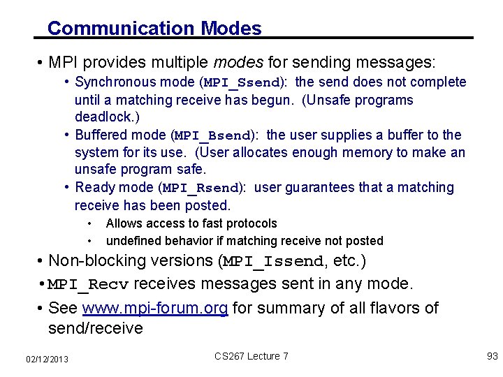
Communication Modes • MPI provides multiple modes for sending messages: • Synchronous mode (MPI_Ssend): the send does not complete until a matching receive has begun. (Unsafe programs deadlock. ) • Buffered mode (MPI_Bsend): the user supplies a buffer to the system for its use. (User allocates enough memory to make an unsafe program safe. • Ready mode (MPI_Rsend): user guarantees that a matching receive has been posted. • • Allows access to fast protocols undefined behavior if matching receive not posted • Non-blocking versions (MPI_Issend, etc. ) • MPI_Recv receives messages sent in any mode. • See www. mpi-forum. org for summary of all flavors of send/receive 02/12/2013 CS 267 Lecture 7 93

Experience and Hybrid Programming CS 267 Lecture 7 99

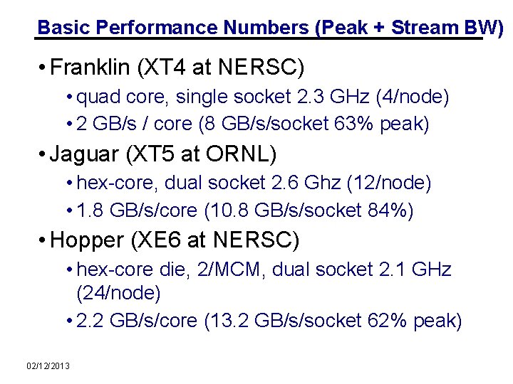
Basic Performance Numbers (Peak + Stream BW) • Franklin (XT 4 at NERSC) • quad core, single socket 2. 3 GHz (4/node) • 2 GB/s / core (8 GB/s/socket 63% peak) • Jaguar (XT 5 at ORNL) • hex-core, dual socket 2. 6 Ghz (12/node) • 1. 8 GB/s/core (10. 8 GB/s/socket 84%) • Hopper (XE 6 at NERSC) • hex-core die, 2/MCM, dual socket 2. 1 GHz (24/node) • 2. 2 GB/s/core (13. 2 GB/s/socket 62% peak) 02/12/2013

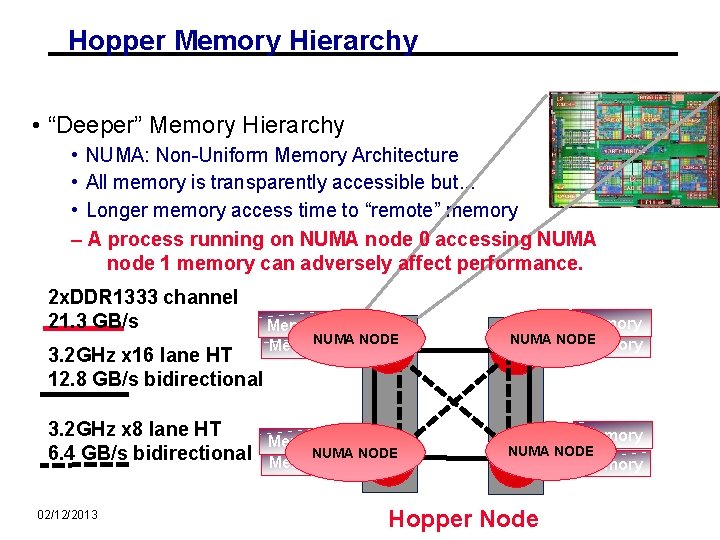
Hopper Memory Hierarchy • “Deeper” Memory Hierarchy • NUMA: Non-Uniform Memory Architecture • All memory is transparently accessible but. . . • Longer memory access time to “remote” memory – A process running on NUMA node 0 accessing NUMA node 1 memory can adversely affect performance. 2 x. DDR 1333 channel 21. 3 GB/s 3. 2 GHz x 16 lane HT 12. 8 GB/s bidirectional 3. 2 GHz x 8 lane HT 6. 4 GB/s bidirectional 02/12/2013 Memory NUMA NODE Memory P 0 Memory NUMA NODE P 1 Memory NUMA NODE Memory P 2 Memory NUMA NODE P 3 Memory Hopper Node

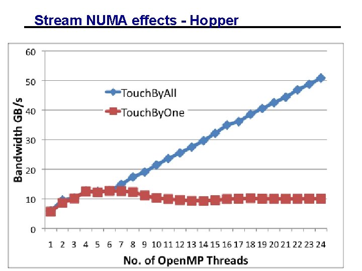
Stream NUMA effects - Hopper 02/12/2013

Stream Benchmark double a[N], b[N], c[N]; ……. #pragma omp parallel for (j=0; j<Vector. Size; j++) { a[j] = 1. 0; b[j] = 2. 0; c[j] = 0. 0; } #pragma omp parallel for (j=0; j<Vector. Size; j++) { a[j]=b[j]+d*c[j]; } … 02/12/2013

MPI Bandwidth and Latency • Franklin & Jaguar – Seastar 2 • ~7 us MPI latency • 1. 6 GB/s/node • 0. 4 GB/s/core Franklin 0. 13 GB/s/core Jaguar • Hopper – Gemini • 1. 6 us MPI latency • 3. 5 GB/s (or 6. 0 GB/s with 2 MB pages) • 0. 14 (0. 5) GB/s/core • Other differences between networks • Gemini has better fault tolerance • Hopper also additional fault tolerance features 02/12/2013

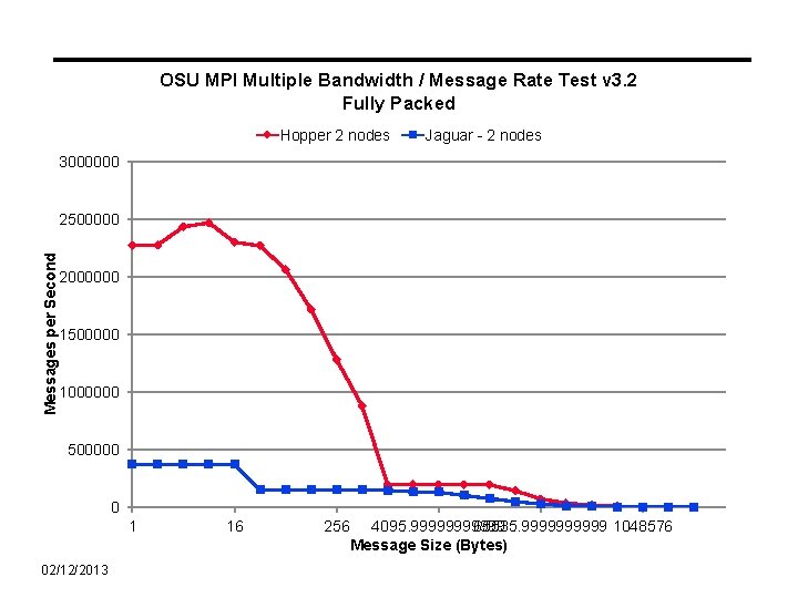
OSU MPI Multiple Bandwidth / Message Rate Test v 3. 2 Fully Packed Hopper 2 nodes Jaguar - 2 nodes 3000000 Messages per Second 2500000 2000000 1500000 1000000 500000 0 1 02/12/2013 16 256 4095. 999999 65535. 99999 1048576 Message Size (Bytes)

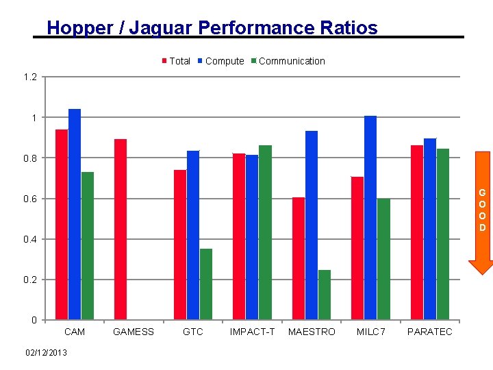
Hopper / Jaguar Performance Ratios Total Compute Communication 1. 2 1 0. 8 G O O D 0. 6 0. 4 0. 2 0 CAM 02/12/2013 GAMESS GTC IMPACT-T MAESTRO MILC 7 PARATEC

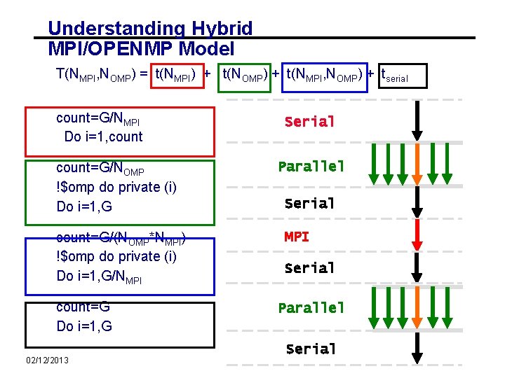
Understanding Hybrid MPI/OPENMP Model T(NMPI, NOMP) = t(NMPI) + t(NOMP) + t(NMPI, NOMP) + tserial count=G/NMPI Do i=1, count=G/NOMP !$omp do private (i) Do i=1, G count=G/(NOMP*NMPI) !$omp do private (i) Do i=1, G/NMPI count=G Do i=1, G 02/12/2013 Serial Parallel Serial MPI Serial Parallel Serial

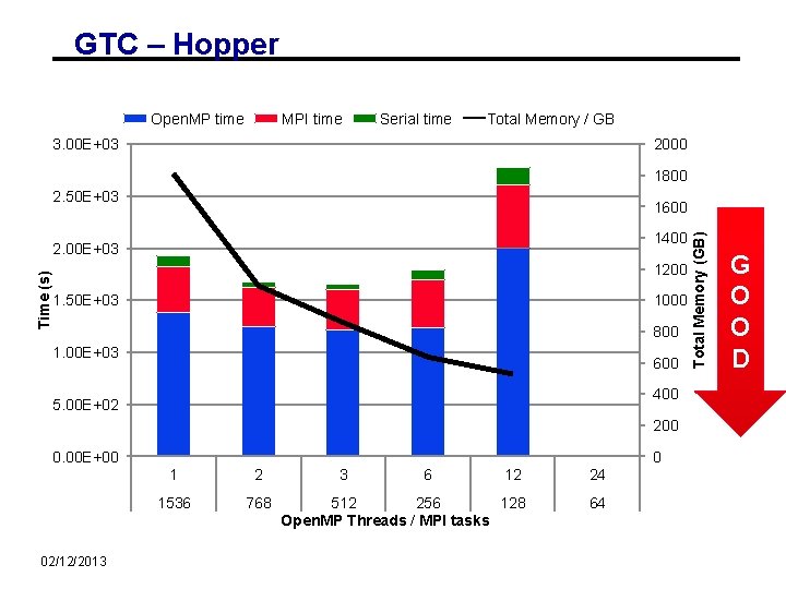
GTC – Hopper Open. MP time MPI time Serial time Total Memory / GB 3. 00 E+03 2000 1800 2. 50 E+03 1400 Time (s) 2. 00 E+03 1200 1. 50 E+03 1000 800 1. 00 E+03 600 400 5. 00 E+02 200 0. 00 E+00 02/12/2013 0 1 2 1536 768 3 6 12 24 512 256 128 Open. MP Threads / MPI tasks 64 Total Memory (GB) 1600 G O O D

Backup Slides (Implementing MPI) 109 CS 267 Lecture 7

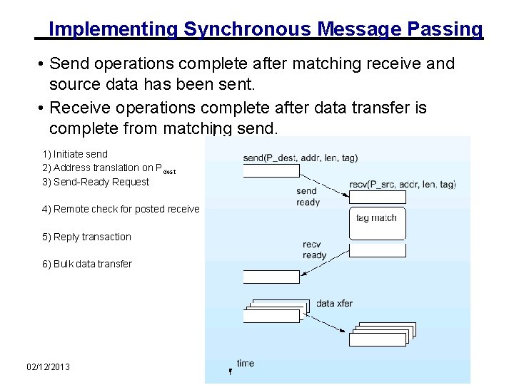
Implementing Synchronous Message Passing • Send operations complete after matching receive and source data has been sent. • Receive operations complete after data transfer is complete from matching send. 1) Initiate send 2) Address translation on Pdest 3) Send-Ready Request source destination send (P dest, addr, length, tag) rcv(Psource, addr, length, tag) send-rdy-request 4) Remote check for posted receive tag match 5) Reply transaction receive-rdy-reply 6) Bulk data transfer data-xfer 02/12/2013 CS 267 Lecture 7 110

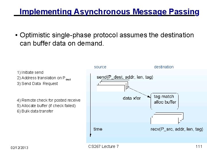
Implementing Asynchronous Message Passing • Optimistic single-phase protocol assumes the destination can buffer data on demand. 1) Initiate send 2) Address translation on Pdest 3) Send Data Request source send (P dest, addr, length, tag) destination data-xfer-request tag match allocate 4) Remote check for posted receive 5) Allocate buffer (if check failed) 6) Bulk data transfer rcv(P source, addr, length, tag) 02/12/2013 CS 267 Lecture 7 111

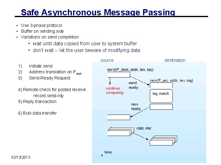
Safe Asynchronous Message Passing • Use 3 -phase protocol • Buffer on sending side • Variations on send completion • wait until data copied from user to system buffer • don’t wait -- let the user beware of modifying data source 1) 2) 3) Initiate send Address translation on Pdest Send-Ready Request 4) Remote check for posted receive record send-rdy 5) Reply transaction destination send-rdy-request return and continue computing tag match receive-rdy-reply 6) Bulk data transfer 02/12/2013 CS 267 Lecture 7 112