Distributed Inference and Query Processing for RFID Tracking
Distributed Inference and Query Processing for RFID Tracking and Monitoring Zhao Cao*, Charles Sutton+, Yanlei Diao*, Prashant Shenoy* *University of Massachusetts, Amherst +University of Edinburgh
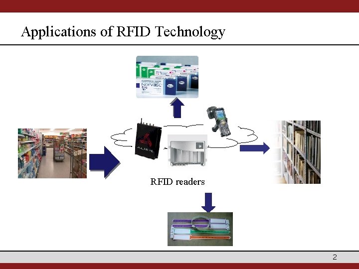
Applications of RFID Technology RFID readers 2
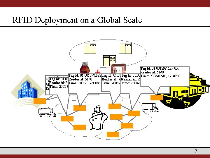
RFID Deployment on a Global Scale + Tag id: 01. 001298. 6 EF. 0 A Reader id: 5140 Tag id: 01. 001298. 6 EF. 0 A Time: 2008 -02 -10, 12: 40: 00 Tag id: 01. 001298. 6 EF. 0 A Tag 01. 001298. 6 EF. 0 A Reader id: 5140 Reader id: 6647 Reader id: 7990 Time: 2008 -01 -12, 14: 30: 00 Reader id: 3478 Time: 2008 -01 -21 08: 15: 00 Time: 2008 -01 -30 Time: 15: 00 2008 -02 -04, 09: 10: 00 Manufacturer: X Ltd. Time: 2008 -01 -15, 06: 10: 00 Expiration date: Oct 2011 3
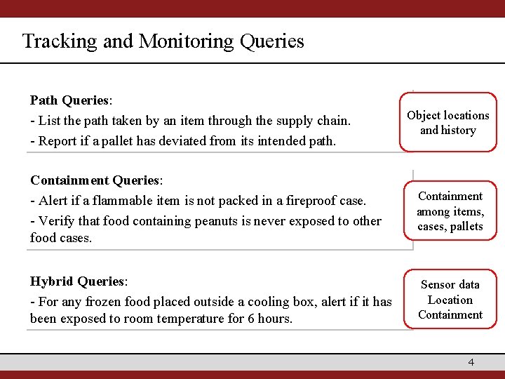
Tracking and Monitoring Queries Path Queries: - List the path taken by an item through the supply chain. - Report if a pallet has deviated from its intended path. Object locations and history Containment Queries: - Alert if a flammable item is not packed in a fireproof case. - Verify that food containing peanuts is never exposed to other food cases. Containment among items, cases, pallets Hybrid Queries: - For any frozen food placed outside a cooling box, alert if it has been exposed to room temperature for 6 hours. Sensor data Location Containment 4
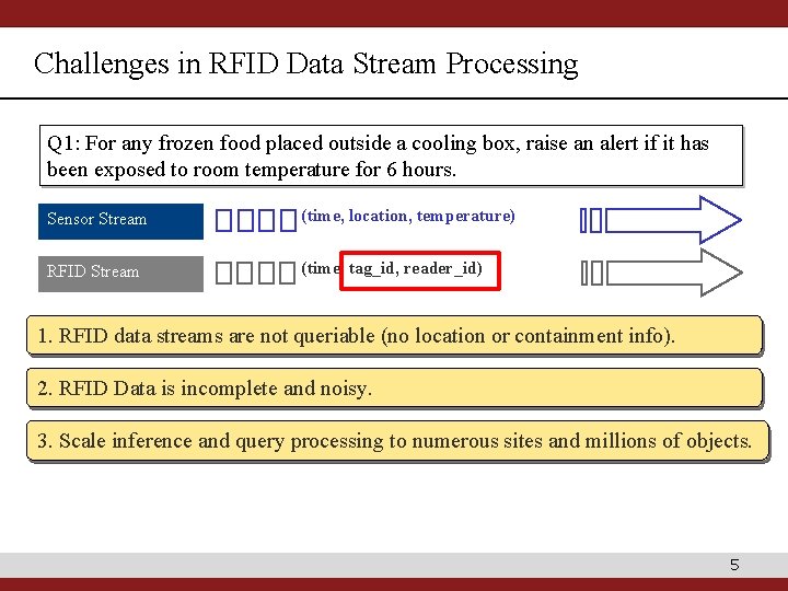
Challenges in RFID Data Stream Processing Q 1: For any frozen food placed outside a cooling box, raise an alert if it has been exposed to room temperature for 6 hours. Sensor Stream (time, location, temperature) RFID Stream (time, tag_id, reader_id) 1. RFID data streams are not queriable (no location or containment info). 2. RFID Data is incomplete and noisy. 3. Scale inference and to numerous sites and millions of objects. 1 query processing 2 1 2 3 Locations: Missing 4 F E 5 6 D Overlapped 3 4 F E 4 5 6 D 5
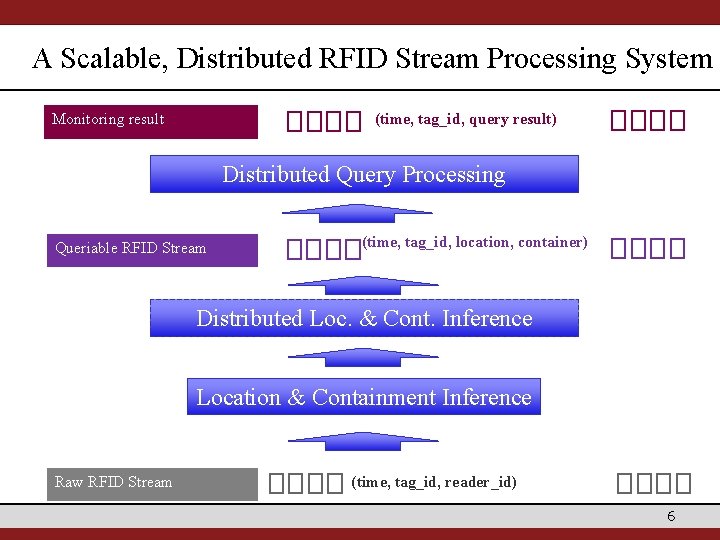
A Scalable, Distributed RFID Stream Processing System Monitoring result (time, tag_id, query result) Distributed Query Processing Queriable RFID Stream (time, tag_id, location, container) Distributed Loc. & Cont. Inference Location & Containment Inference Raw RFID Stream (time, tag_id, reader_id) 6

I. Location and Containment Inference – Intuition Time t=1 Cases Items 1 3 t=2 2 4 5 t=3 1 6 Reader location: A 3 2 4 B Containment Inference: Co-location history Item 5 is contained in case 2 5 1 6 C t=4 3 2 4 D Iterative procedure E 5 1 6 C 3 2 4 F 5 E 6 D Location Inference: Smoothing over containment Case 2 is in Location C at t=3 Item 6 is contained in case 2 Containment Changes: Change point detection Containment between case 1 and item 4 has changed 7
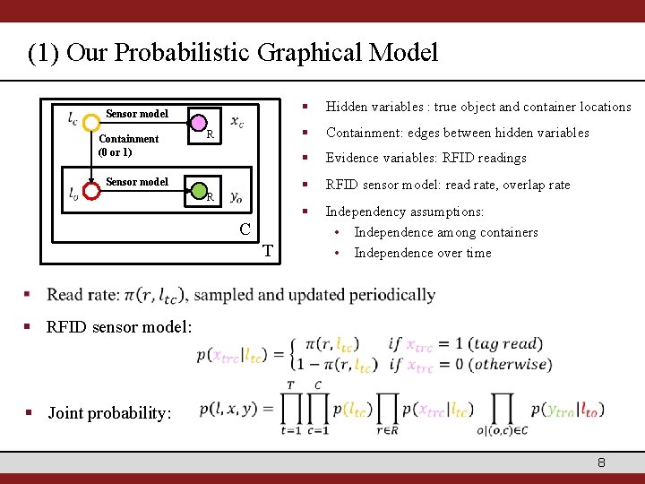
(1) Our Probabilistic Graphical Model Sensor model Containment (0 or 1) R Sensor model R C T § Hidden variables : true object and container locations § Containment: edges between hidden variables § Evidence variables: RFID readings § RFID sensor model: read rate, overlap rate § Independency assumptions: • Independence among containers • Independence over time § RFID sensor model: § Joint probability: 8
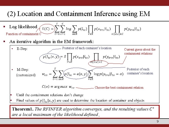
(2) Location and Containment Inference using EM § Log likelihood Function of containment C § An iterative algorithm in the EM framework: • E-Step: • M-Step: (customized) Posterior of each container’s location Current guess about the containment relations Posterior of each container’s location Choose the best containment relation . 9
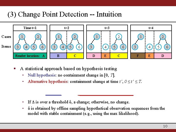
(3) Change Point Detection -- Intuition Time t=1 Cases Items 1 3 t=2 2 4 5 t=3 1 6 Reader location: A 3 2 4 B 5 1 6 C t=4 3 2 4 D 5 E 1 6 C 3 2 4 F E 5 6 D § A statistical approach based on hypothesis testing • Null hypothesis: no containment change in [0, T]. • Alternative hypothesis: containment change at time t’, 0 ≤ t’ ≤ T. • If Δ is over a threshold δ, a change; otherwise, no change. • δ is obtained by offline sampling hypothetical observation sequences from the model with stable containment (e. g. , using the max likelihood). 10
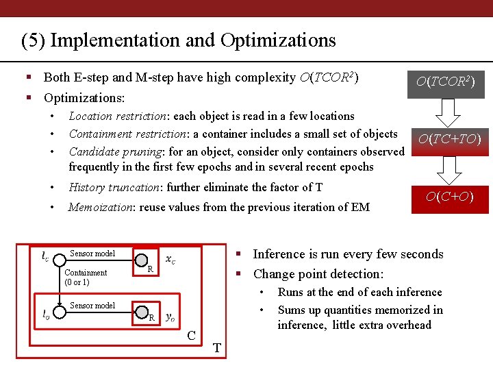
(5) Implementation and Optimizations § Both E-step and M-step have high complexity O(TCOR 2) § Optimizations: • • • Location restriction: each object is read in a few locations Containment restriction: a container includes a small set of objects Candidate pruning: for an object, consider only containers observed frequently in the first few epochs and in several recent epochs • History truncation: further eliminate the factor of T • Memoization: reuse values from the previous iteration of EM O(TC+TO) O(C+O) § Inference is run every few seconds § Change point detection: Sensor model Containment (0 or 1) O(TCOR 2) R • • Sensor model R C T Runs at the end of each inference Sums up quantities memorized in inference, little extra overhead 11
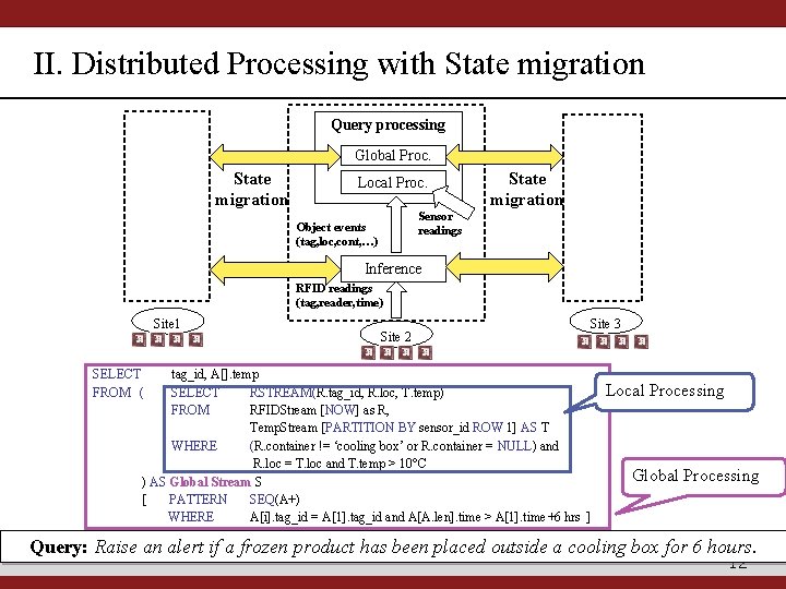
II. Distributed Processing with State migration Query processing Global Proc. State migration Local Proc. State migration Sensor readings Object events (tag, loc, cont, …) Inference RFID readings (tag, reader, time) Site 1 SELECT FROM ( Site 2 Site 3 tag_id, A[]. temp SELECT RSTREAM(R. tag_id, R. loc, T. temp) FROM RFIDStream [NOW] as R, Temp. Stream [PARTITION BY sensor_id ROW 1] AS T WHERE (R. container != ‘cooling box’ or R. container = NULL) and R. loc = T. loc and T. temp > 10°C ) AS Global Stream S [ PATTERN SEQ(A+) WHERE A[i]. tag_id = A[1]. tag_id and A[A. len]. time > A[1]. time+6 hrs ] Local Processing Global Processing Query: Raise an alert if a frozen product has been placed outside a cooling box for 6 hours. 12
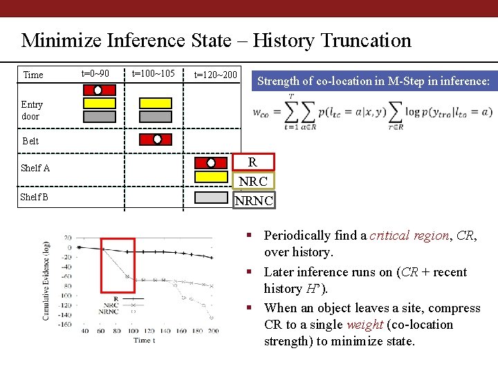
Minimize Inference State – History Truncation Time t=0~90 t=100~105 t=120~200 Strength of co-location in M-Step in inference: Entry door Belt Shelf A Shelf B R NRC NRNC § Periodically find a critical region, CR, over history. § Later inference runs on (CR + recent history H’). § When an object leaves a site, compress CR to a single weight (co-location strength) to minimize state. 13
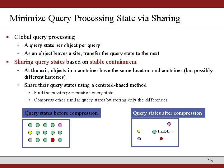
Minimize Query Processing State via Sharing § Global query processing • A query state per object per query • As an object leaves a site, transfer the query state to the next § Sharing query states based on stable containment • At the exit, objects in a container have the same location and container (but possibly different histories) • Share their query states using a centroid-based method • Find the most representative query state • Compress other similar query states by storing only the differences Query states before compression Query states after compression [1, 2, 3, 4…] 15
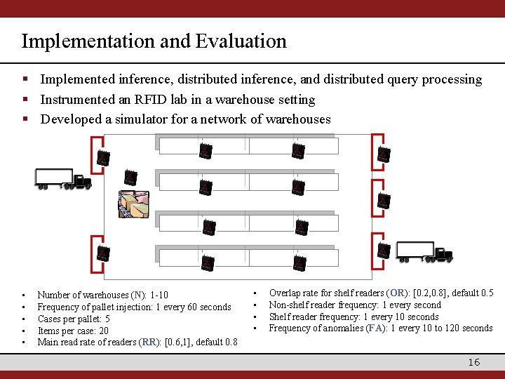
Implementation and Evaluation § Implemented inference, distributed inference, and distributed query processing § Instrumented an RFID lab in a warehouse setting § Developed a simulator for a network of warehouses • • • Number of warehouses (N): 1 -10 Frequency of pallet injection: 1 every 60 seconds Cases per pallet: 5 Items per case: 20 Main read rate of readers (RR): [0. 6, 1], default 0. 8 • • Overlap rate for shelf readers (OR): [0. 2, 0. 8], default 0. 5 Non-shelf reader frequency: 1 every second Shelf reader frequency: 1 every 10 seconds Frequency of anomalies (FA): 1 every 10 to 120 seconds 16
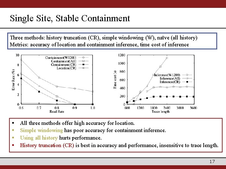
Single Site, Stable Containment Three methods: history truncation (CR), simple windowing (W), naïve (all history) Metrics: accuracy of location and containment inference, time cost of inference § § All three methods offer high accuracy for location. Simple windowing has poor accuracy for containment inference. Using all history hurts performance. History truncation (CR) is best in accuracy and performance, insensitive to trace length. 17
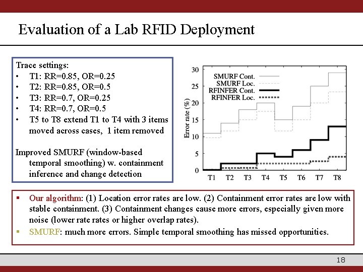
Evaluation of a Lab RFID Deployment Trace settings: • T 1: RR=0. 85, OR=0. 25 • T 2: RR=0. 85, OR=0. 5 • T 3: RR=0. 7, OR=0. 25 • T 4: RR=0. 7, OR=0. 5 • T 5 to T 8 extend T 1 to T 4 with 3 items moved across cases, 1 item removed Improved SMURF (window-based temporal smoothing) w. containment inference and change detection § § Our algorithm: (1) Location error rates are low. (2) Containment error rates are low with stable containment. (3) Containment changes cause more errors, especially given more noise (lower rates or higher overlap rates). SMURF: much more errors. Simple temporal smoothing has missed opportunities. 18
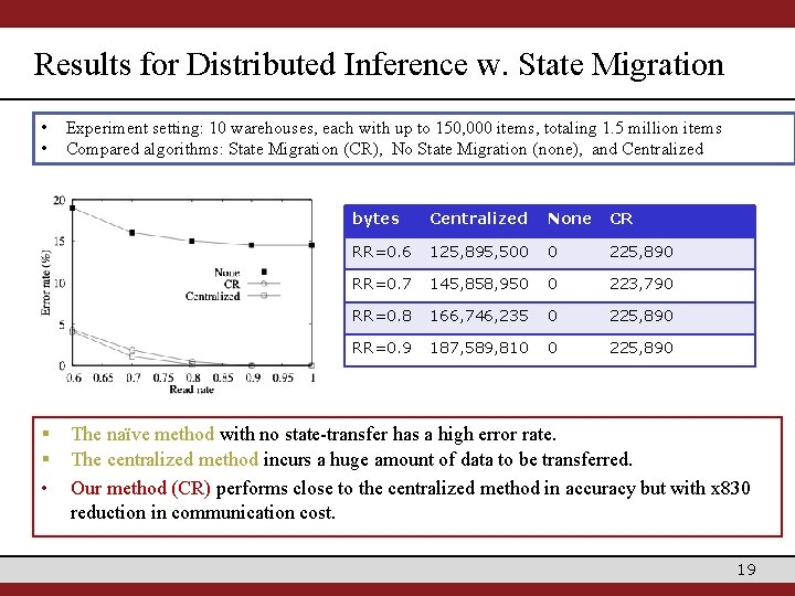
Results for Distributed Inference w. State Migration • • § § • Experiment setting: 10 warehouses, each with up to 150, 000 items, totaling 1. 5 million items Compared algorithms: State Migration (CR), No State Migration (none), and Centralized bytes Centralized None CR RR=0. 6 125, 895, 500 0 225, 890 RR=0. 7 145, 858, 950 0 223, 790 RR=0. 8 166, 746, 235 0 225, 890 RR=0. 9 187, 589, 810 0 225, 890 The naïve method with no state-transfer has a high error rate. The centralized method incurs a huge amount of data to be transferred. Our method (CR) performs close to the centralized method in accuracy but with x 830 reduction in communication cost. 19
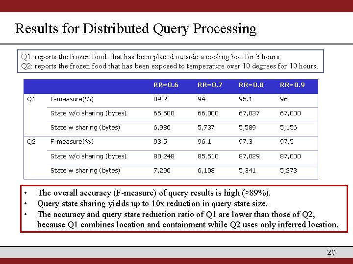
Results for Distributed Query Processing Q 1: reports the frozen food that has been placed outside a cooling box for 3 hours. Q 2: reports the frozen food that has been exposed to temperature over 10 degrees for 10 hours. Q 1 Q 2 • • • RR=0. 6 RR=0. 7 RR=0. 8 RR=0. 9 F-measure(%) 89. 2 94 95. 1 96 State w/o sharing (bytes) 65, 500 66, 000 67, 037 67, 000 State w sharing (bytes) 6, 986 5, 737 5, 589 5, 156 F-measure(%) 93. 5 96. 1 97. 3 97. 5 State w/o sharing (bytes) 80, 248 85, 510 87, 029 87, 000 State w sharing (bytes) 7, 296 6, 108 5, 341 5, 273 The overall accuracy (F-measure) of query results is high (>89%). Query state sharing yields up to 10 x reduction in query state size. The accuracy and query state reduction ratio of Q 1 are lower than those of Q 2, because Q 1 combines location and containment while Q 2 uses only inferred location. 20
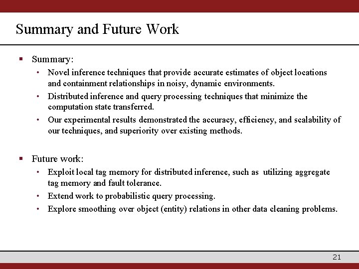
Summary and Future Work § Summary: • Novel inference techniques that provide accurate estimates of object locations and containment relationships in noisy, dynamic environments. • Distributed inference and query processing techniques that minimize the computation state transferred. • Our experimental results demonstrated the accuracy, efficiency, and scalability of our techniques, and superiority over existing methods. § Future work: • Exploit local tag memory for distributed inference, such as utilizing aggregate tag memory and fault tolerance. • Extend work to probabilistic query processing. • Explore smoothing over object (entity) relations in other data cleaning problems. 21

Thank You! 22
- Slides: 21