Distributed Hydrologic modeling and Problembased learning techniques using

Distributed Hydrologic modeling and Problem-based learning techniques using HPC resources Case of Logan River catchment, Utah David Baron Tseganeh Z Gichamo USU - Hydroinformatics November 29, 2012

Objectives � Testing and prototyping the processes involved in UEBGrid model instantiation for a particular watershed, so that simulation will be executed in HPC Grid using the CI-Water Cyber-collaboratory. � Applying it for interactive web-based hydrologic instruction using problem-based learning techniques � Generalizing the insight gained through this exercise to other hydrological models

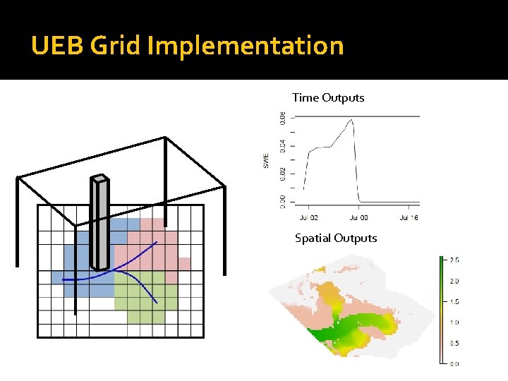
UEB Grid Implementation Time Outputs Spatial Outputs

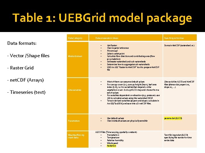
Table 1: UEBGrid model package Data Category Data formats: - Vector /Shape files Model domain – – – – - Raster Grid - net. CDF (Arrays) - Timeseries (text) Data preparation Steps – – Site variables – – Parameters Weather/forcing input data – – Resulting outcomes Get Raster Check spatial reference Pit removal Select outlet point Calculate flow direction and contributing area (flow accumulation) Delineate watershed and sub-watersheds Determine how to aggregate sub-watersheds USE Arc. GIS “Raster to Net. CDF” tool to prepare Net. CDF file Domain Net. CDF (watershed. nc) Most of them can assume default values For canopy cover (cc), canopy height (hcan), leaf area index (LAI), i. e. for variables that depend on the vegetation cover: look up NLCD map and choose from a set of values For variables dependent on elevation (e. g. pressure): use GIS to calculate values using the watershed DEM Terrain derived variables (aspect and slope): calculate in Arc. GIS/Tau. DEM, and save into 2 D net. CDF files. Site variables ASCII and Net. CDF files (sitevar. dat, aspect. nc, slope. nc, …) Use default values Check default values are physically sensible params. dat (ASCII) ASCII Files (Time varying, spatially constant) – Precipitation – Temperature – Relative humidity – Wind speed – Radiation Text file input. dat (ASCII) specifying file names for time series data

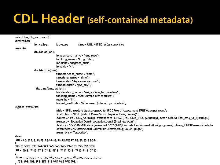
net. CDF � net. CDF: network Common Data Format Array (Multi-dimensional) Data format Set of libraries and tools Self-descriptive, Platform independent, Easy to sub-set and append Model need to be linked with net. CDF Libraries Tools: ncgen, ncdump

CDL Header (self-contained metadata) netcdf tos_O 1_2001 -2002 { dimensions: lon = 180 ; lat = 170 ; time = UNLIMITED ; // (24 currently); variables: double lon(lon) ; lon: standard_name = "longitude" ; lon: long_name = "longitude" ; lon: units = "degrees_east" ; lon: axis = "X" ; double time(time) ; time: standard_name = "time" ; time: long_name = "time" ; time: units = "days since 2001 -1 -1" ; time: calendar = "360_day" ; float tos(time, lat, lon) ; tos: standard_name = "sea_surface_temperature" ; tos: long_name = "Sea Surface Temperature" ; tos: units = "K" ; tos: cell_methods = "time: mean (interval: 30 minutes)" ; // global attributes: : title = "IPSL model output prepared for IPCC Fourth Assessment SRES A 2 experiment" ; : institution = "IPSL (Institut Pierre Simon Laplace, Paris, France)" ; : source = "IPSL-CM 4_v 1 (2003) : atmosphere : LMDZ (IPSL-CM 4_IPCC, 96 x 71 x 19) ; ocean ORCA 2 (ipsl_cm 4_v 1_8, 2 x 2 L 31); : contact = "Sebastien Denvil, sebastien. denvil@ipsl. jussieu. fr" ; : history = "YYYY/MM/JJ: data generated; YYYY/MM/JJ+1 data transformed At 16: 37: 23 on 01/11/2005, CMOR rewrote data to : references = "Dufresne et al, Journal of Climate, 2015, vol XX, p 136" ; : comment = "Test drive" ; data: lon = 1, 3, 5, 7, 9, 11, 13, 15, 17, 19, 21, 23, 25, 27, 29, 31, 33, 35, 37, // 333, 335, 337, 339, 341, 343, 345, 347, 349, 351, 353, 355, 357, 359 ; lat = -79. 5, -78. 5, -77. 5, -76. 5, -75. 5, -74. 5, -73. 5, -72. 5, -71. 5, -70. 5, // time = 15, 45, 75, 105, 135, 165, 195, 225, 255, 285, 315, 345, 375, 405, 435, 465, 495, 525, 555, 585, 615, 645, 675, 705 ;

Aspect in IDV vs Arc-GIS

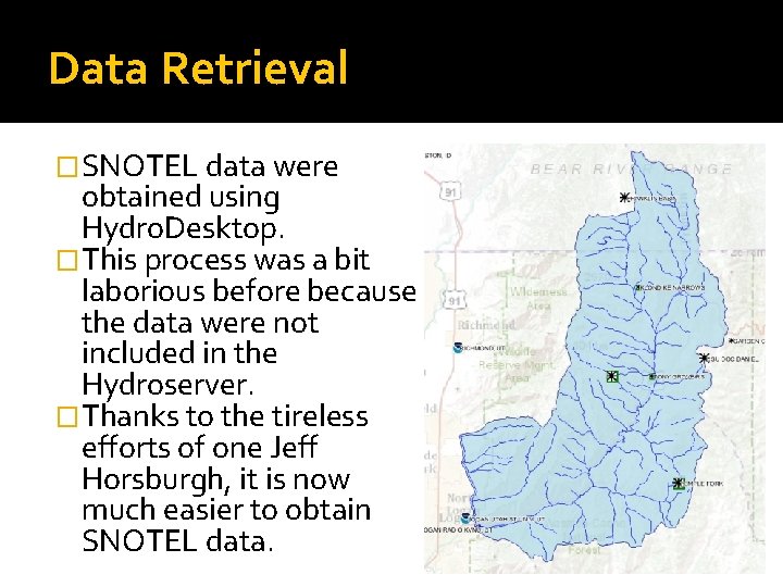
Data Retrieval �SNOTEL data were obtained using Hydro. Desktop. �This process was a bit laborious before because the data were not included in the Hydroserver. �Thanks to the tireless efforts of one Jeff Horsburgh, it is now much easier to obtain SNOTEL data.

Educational Applications � Modules are currently being created using real and model data. � These modules will provide an online laboratory for students to learn hydrology. � The modules will follow a problem-based learning model.

Educational Applications (2) �Using the data generated by the model, we are creating modules that will: Teach students about the sustainability of water supplies. Show students how human interactions affect the hydrology of a river basin or watershed. Teach students risk assessment and abatement techniques associated with protecting properties from flooding. *

Educational Applications – LDC �One of the study areas for the problem-based modules is Logan Dry Canyon (LDC). �This is a small watershed (about 3. 5 sq. mi. ) �There are no SNOTEL stations or rain gauges within the watershed. �An attempt was made to use PRISM as a source but the spatial and temporal resolution proved to be too large.

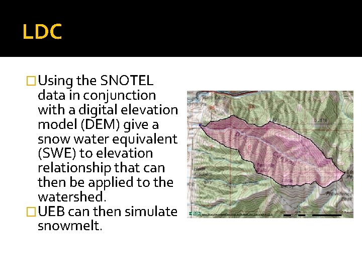
LDC �Using the SNOTEL data in conjunction with a digital elevation model (DEM) give a snow water equivalent (SWE) to elevation relationship that can then be applied to the watershed. �UEB can then simulate snowmelt.

LDC �The end goal of the LDC module is to get the students to design a flood and then design a structure or method to minimize or prevent damage to nearby properties. �Methods used will include calculating a hyetograph and a hydrograph for the watershed that can then be used to determine the flood risk.

References [1] J. C. Refsgaard, M. B. Abbott, "The Role of Distributed Hydrological Modelling in Water Resources Management. " Distributed Hydrological Modelling, 1– 16, 1996. [2] D. G. Tarboton, T. G. Chowdhury and T. H. Jackson, "A Spatially Distributed Energy Balance Snowmelt Model, " in Biogeochemistry of Seasonally Snow-Covered Catchments, ed. K. A. Tonnessen et al. , Proceedings of a Boulder Symposium, IAHS Publ. no. 228, p. 141 -155, July 3 -14, 1995. [3] V. Mahat and D. G. Tarboton, (2012), "Canopy radiation transmission for an energy balance snowmelt model, " Water Resources Research vol. 48, W 01534. [4] Y. Qu and C. J. Duffy, “A semidiscrete finite volume formulation for multiprocess watershed simulation”, Water Resources Research Vol. 43, W 08419, 2007 [5] C. Shen and M. S. Phanikumar, “A process-based, distributed hydrologic model based on a large-scale method for surface–subsurface coupling”, Advances in Water Resources vol. 33, pp 1524– 1541, 2010 [6] R. K. Rew, G. P. Davis, S. Emmerson and H. Davies, Net. CDF User's Guide for C, An Interface for Data Access, Version 3, April 1997. [7] http: //www. unidata. ucar. edu/software/netcdf/docs/faq. html#whatisit [8] https: //www. hpc. usu. edu/wiki/Getting. Started 2 Job. Scripts#Job. Scripts

Thank you �Questions?