Distances A natural or ideal measure of distance

Distances

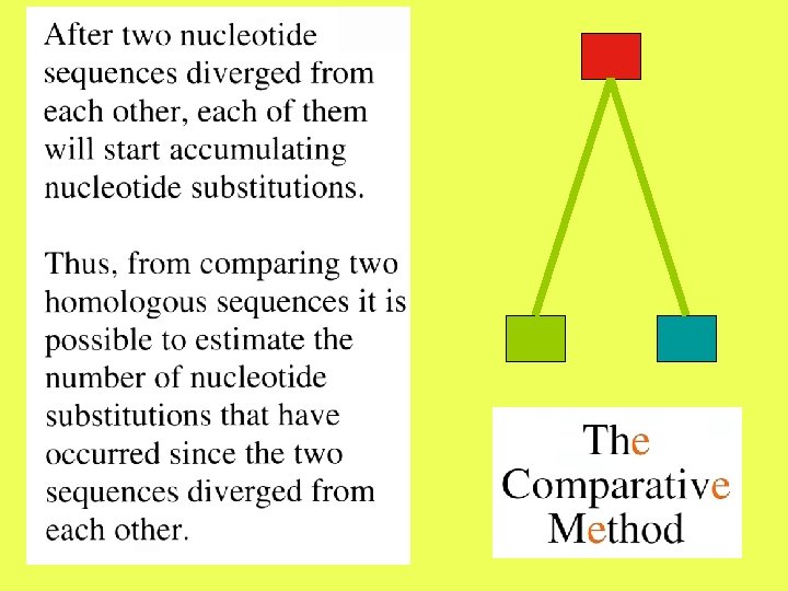
A natural or ideal measure of distance between two sequences should have an evolutionary meaning. One such measure may be the number of nucleotide substitutions that have accumulated in the two sequences since they have diverged from each other.

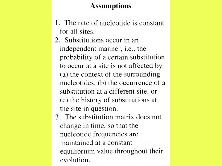
To derive a measure of distance, we need to make several simplifying assumptions regarding the probability of substitution of a nucleotide by another.

Jukes & Cantor one-parameter model

Assumption: • Substitutions occur with equal probabilities among the four nucleotide types.

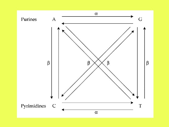
Kimura’s two-parameter model

Assumptions: • The rate of transitional substitution at each nucleotide site is per unit time. • The rate of each type of transversional substitution is per unit time.

NUMBER OF NUCLEOTIDE SUBSTITUTIONS BETWEEN TWO DNA SEQUENCES

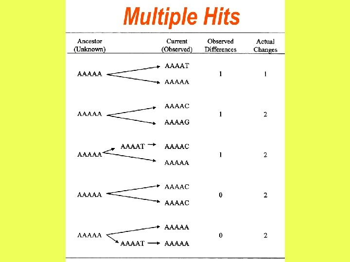
After two nucleotide sequences diverge from each other, each of them will start accumulating nucleotide substitutions. If two sequences of length N differ from each other at n sites, then the proportion of differences, n/N, is referred to as the degree of divergence or Hamming distance. Degrees of divergence are usually expressed as percentages (n/N 100%).

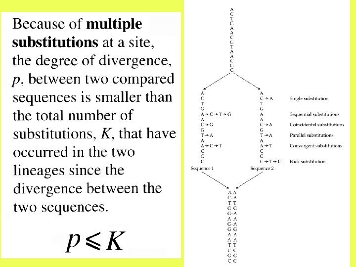
The observed number of differences is likely to be smaller than the actual number of substitutions due to multiple hits at the same site.

13 mutations = 3 differences

Number of substitutions between two noncoding sequences

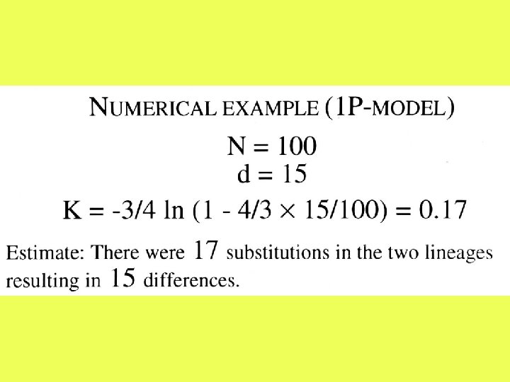
The one-parameter model In this model, it is sufficient to consider only I(t), which is the probability that the nucleotide at a given site at time t is the same in both sequences.

where p is the observed proportion of different nucleotides between the two sequences.

L = number of sites compared in the ungapped alignment between the two sequences.

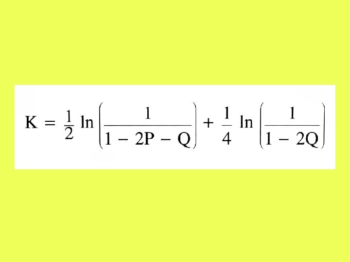
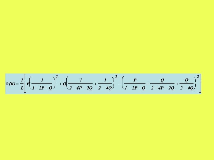
The two-parameter model

The differences between two sequences are classified into transitions and transversions. P = proportion of transitional differences Q = proportion of transversional differences ATCGG ACCCG Q = 0. 2 P = 0. 2

Numerical example (2 P-model)

-Substitution schemes with more than two parameters. - Parameter-free substitution schemes.

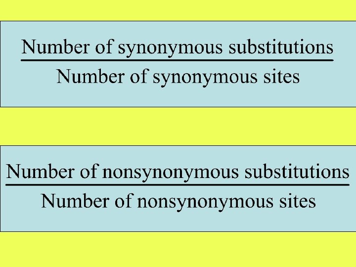
Number of substitutions between two protein-coding genes

Difficulties with denominator: 1. The classification of a site changes with time: For example, the third position of CGG (Arg) is synonymous. However, if the first position changes to T, then the third position of the resulting codon, TGG (Trp), becomes nonsynonymous.

T Trp Nonsynonymous

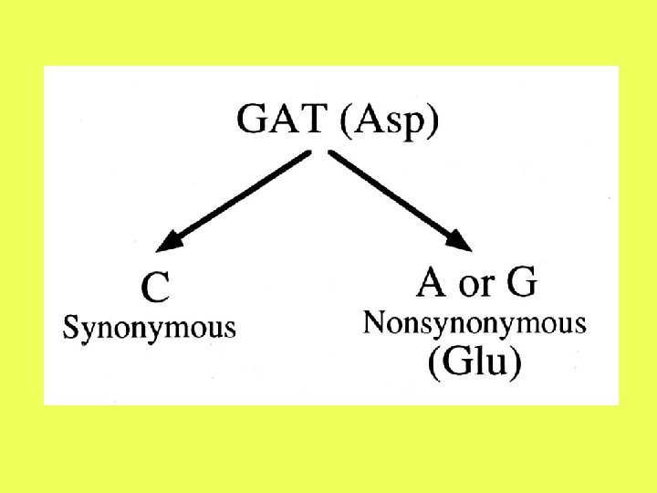
Difficulties with denominator: 2. Many sites are neither completely synonymous nor completely nonsynonymous. For example, a transition in the third position of GAT (Asp) will be synonymous, while a transversion to either GAG or GAA will alter the amino acid.

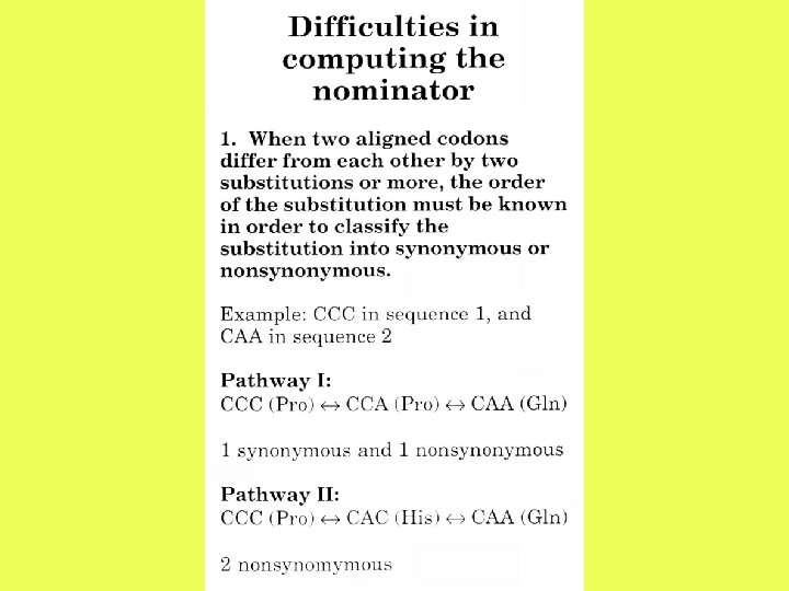
Difficulties with nominator: 1. The classification of the change depends on the order in which the substitutions had occurred.

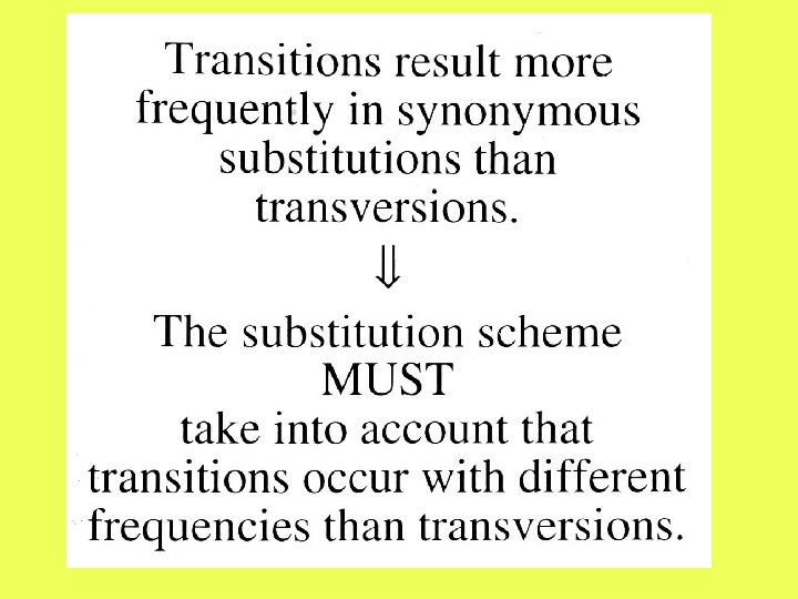
Difficulties with nominator: 2. Transitions occur with different frequencies than transversions. 3. The type of substitution depends on the mutation. Transitions result more frequently in synonymous substitutions than transversions.

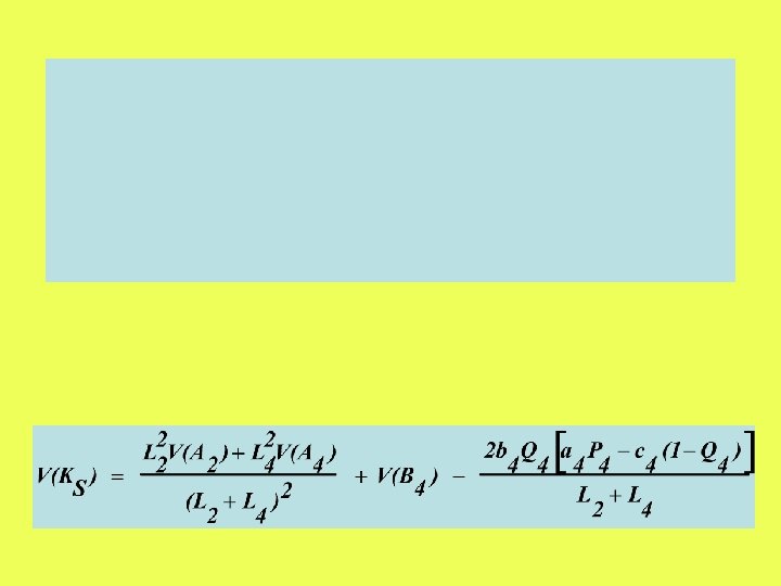
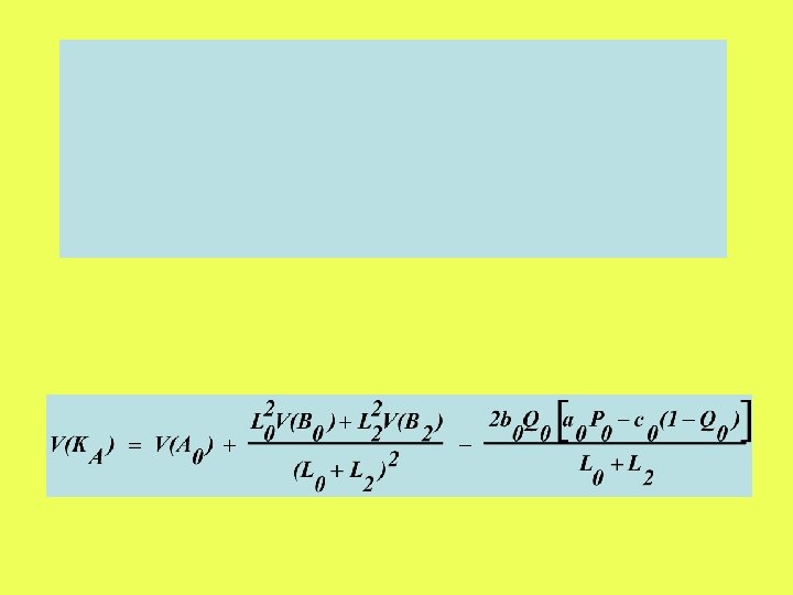
Miyata & Yasunaga (1980) and Nei & Gojobori (1986) method

Step 1: Classify Nucleotides into non-degenerate, twofold and fourfold degenerate sites L 0 L 2 L 4

Number of Amino-Acid Replacements between Two Proteins • The observed proportion of different amino acids between the two sequences (p) is p = n /L • n = number of amino acid differences between the two sequences • L = length of the aligned sequences.

Number of Amino-Acid Replacements between Two Proteins The Poisson model is used to convert p into the number of amino replacements between two sequences (d ): d = - ln(1 – p) The variance of d is estimated as V(d) = p/L (1 – p)

How do you detect adaptive evolution at the genetic level?

Theoretical Expectations Deleterious mutations Neutral mutations Advantageous mutations Overdominant mutations 48

49

50

51

52

53