Dissipative Particle Dynamics Molecular Dynamics why slow MD

Dissipative Particle Dynamics

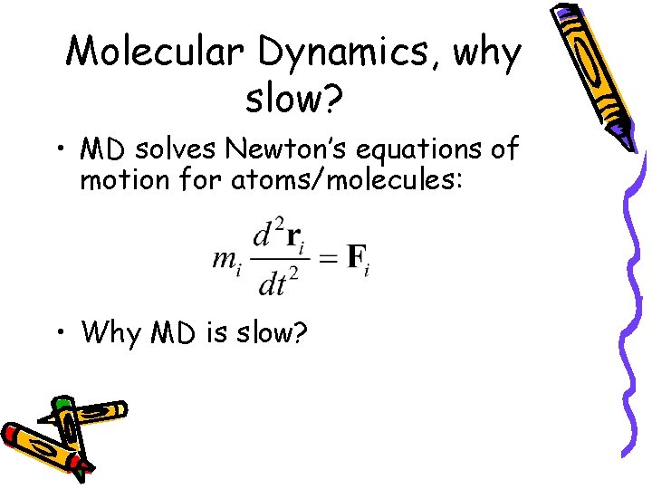
Molecular Dynamics, why slow? • MD solves Newton’s equations of motion for atoms/molecules: • Why MD is slow?

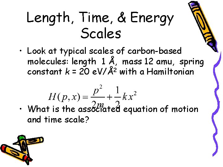
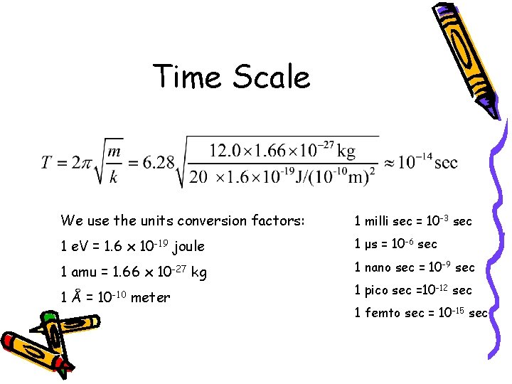
Length, Time, & Energy Scales • Look at typical scales of carbon-based molecules: length 1 Å, mass 12 amu, spring constant k = 20 e. V/Å2 with a Hamiltonian • What is the associated equation of motion and time scale?

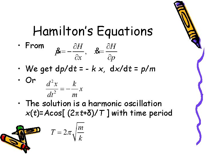
Hamilton’s Equations • From • We get dp/dt = - k x, dx/dt = p/m • Or • The solution is a harmonic oscillation x(t)=Acos[ (2 t+δ)/T ] with time period

Time Scale We use the units conversion factors: 1 milli sec = 10 -3 sec 1 e. V = 1. 6 x 10 -19 joule 1 μs = 10 -6 sec 1 amu = 1. 66 x 10 -27 kg 1 nano sec = 10 -9 sec 1Å= 10 -10 meter 1 pico sec =10 -12 sec 1 femto sec = 10 -15 sec

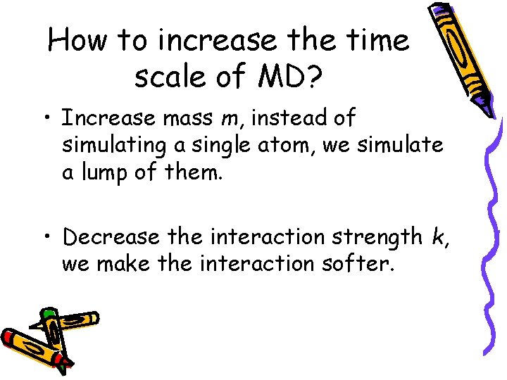
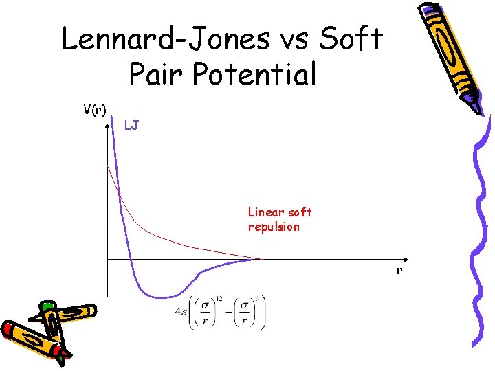
How to increase the time scale of MD? • Increase mass m, instead of simulating a single atom, we simulate a lump of them. • Decrease the interaction strength k, we make the interaction softer.

Lennard-Jones vs Soft Pair Potential V(r) LJ Linear soft repulsion r

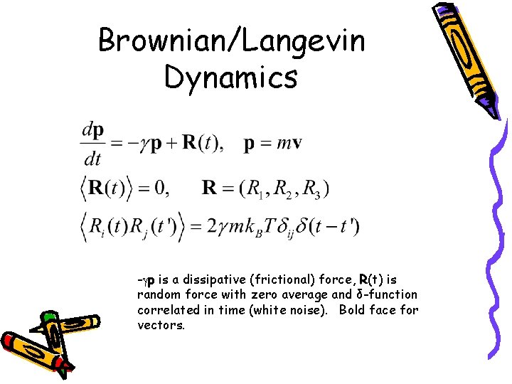
Brownian/Langevin Dynamics - p is a dissipative (frictional) force, R(t) is random force with zero average and δ-function correlated in time (white noise). Bold face for vectors.

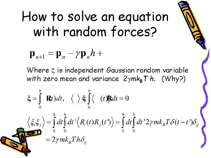
How to solve an equation with random forces? Where is independent Gaussian random variable with zero mean and variance 2 mk. BT h. (Why? )

Statistical Ensembles • Micro-canonical ensemble: fixed particle number, volume, and energy (N, V, E) • Canonical ensemble: fixed particle number, volume, and temperature (N, V, T). Langevin dynamics implements a canonical ensemble.

Dissipative Particle Method • The dissipative particle dynamics was first proposed by Hoogerbrugge and Koelman (1992) for simulating hydrodynamic behavior. It was further improved by Groot and Warren (1997). It is a molecular dynamics with pair forces of three types.

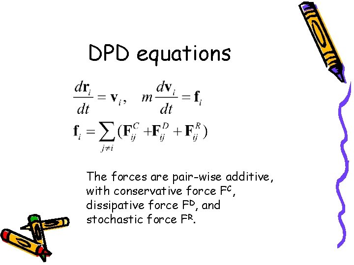
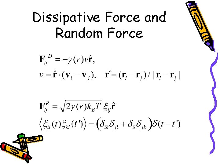
DPD equations The forces are pair-wise additive, with conservative force FC, dissipative force FD, and stochastic force FR.

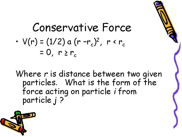
Conservative Force • V(r) = (1/2) a (r –rc)2, r < rc = 0, r ≥ rc Where r is distance between two given particles. What is the form of the force acting on particle i from particle j ?

Dissipative Force and Random Force

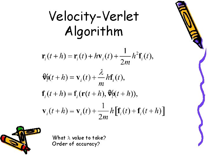
Velocity-Verlet Algorithm What value to take? Order of accuracy?

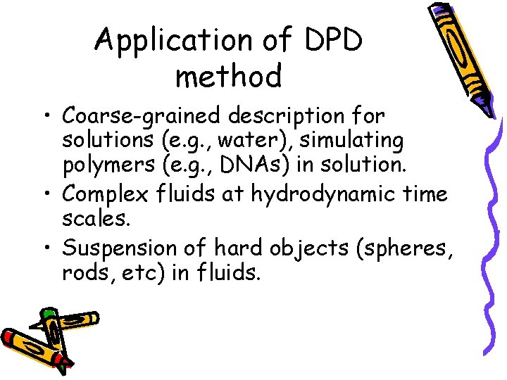
Application of DPD method • Coarse-grained description for solutions (e. g. , water), simulating polymers (e. g. , DNAs) in solution. • Complex fluids at hydrodynamic time scales. • Suspension of hard objects (spheres, rods, etc) in fluids.

Smoothed Particle Hydrodynamics • A typical class of methods where continuum field equations (such as hydrodynamic equations) are simulated using the concept of particles. • The traditional methods was to solve the partial differential equations on a regular grids (in space and time).