Displaying Quantitative Data Histograms Stem and Leaf Plots

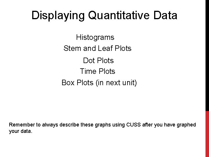
Displaying Quantitative Data Histograms Stem and Leaf Plots Dot Plots Time Plots Box Plots (in next unit) Remember to always describe these graphs using CUSS after you have graphed your data.

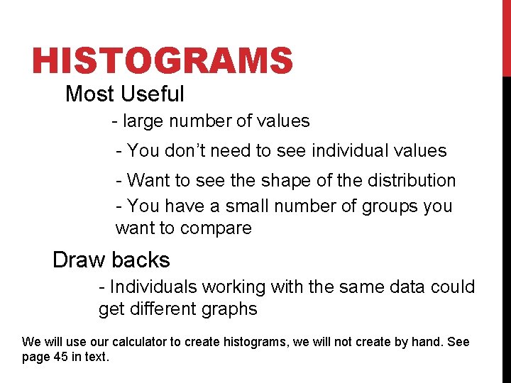
HISTOGRAMS Most Useful - large number of values - You don’t need to see individual values - Want to see the shape of the distribution - You have a small number of groups you want to compare Draw backs - Individuals working with the same data could get different graphs We will use our calculator to create histograms, we will not create by hand. See page 45 in text.

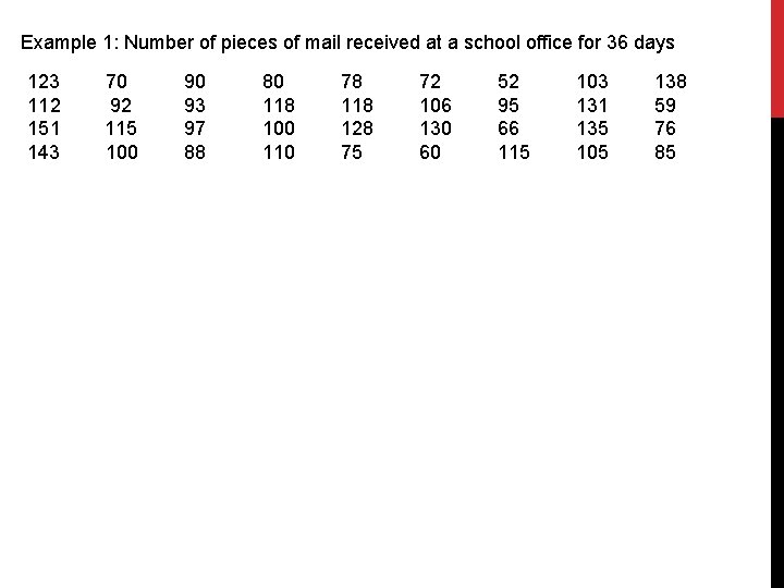
Example 1: Number of pieces of mail received at a school office for 36 days 123 112 151 143 70 92 115 100 90 93 97 88 80 118 100 110 78 118 128 75 72 106 130 60 52 95 66 115 103 131 135 105 138 59 76 85

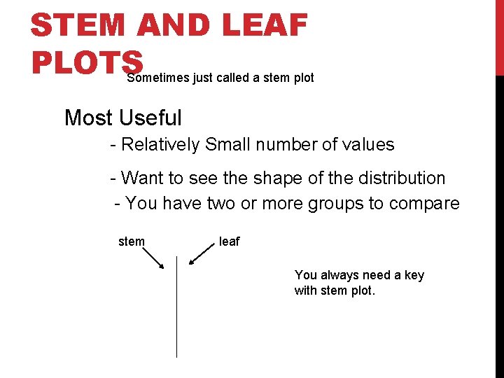
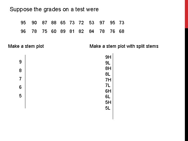
STEM AND LEAF PLOTS Sometimes just called a stem plot Most Useful - Relatively Small number of values - Want to see the shape of the distribution - You have two or more groups to compare stem leaf You always need a key with stem plot.

Suppose the grades on a test were 95 90 87 88 65 73 72 53 97 95 73 96 78 75 60 89 81 82 84 78 76 68 Make a stem plot 9 8 7 6 5 Make a stem plot with split stems 9 H 9 L 8 H 8 L 7 H 7 L 6 H 6 L 5 H 5 L

DOT PLOTS Most Useful - Small number of values - Want to see individual values - Want to see the shape of the distribution - You have a small number of groups you want to compare Let’s make a dot plot for the number of movies we saw this summer.

TIME PLOTS - Type of dot plot - Plot data in order according to time See an example of a Time plot on page 48 in text.

QUANTITATIVE DATA CONDITION The data are values of a quantitative variable whose units are known. Although a bar chart and a histogram may look alike, they are not the same display. You CANNOT display categorical data using a histogram or quantitative data in a bar chart. Always check the type of data before chosing your display method.

SHAPE OF DISTRIBUTION When you describe a distribution, you should talk about three things: Its Shape Its Center Its Spread CUSS

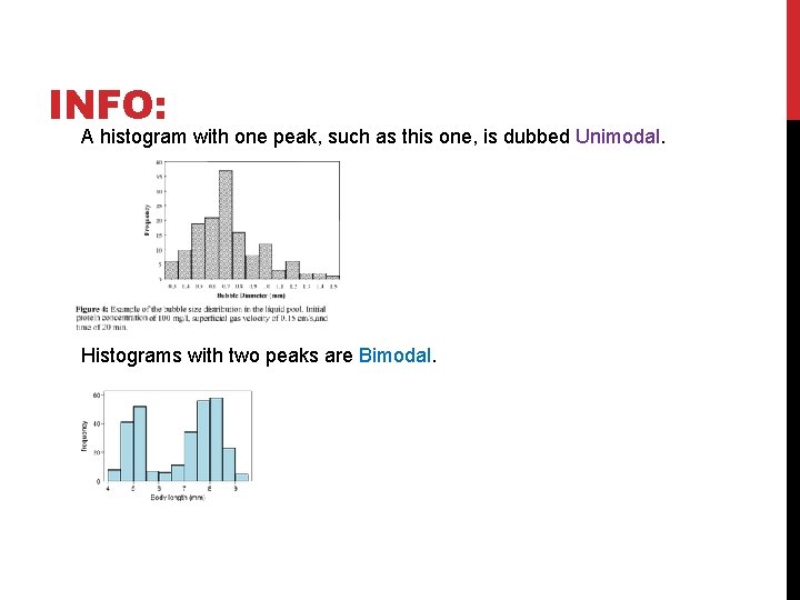
ITS SHAPE Does the histogram have a single central hump? Or does it have several humps? These humps are called modes.

INFO: A histogram with one peak, such as this one, is dubbed Unimodal. Histograms with two peaks are Bimodal.

INFO: Histograms that do not have an obvious mode (the bars are about the same length) are called Uniform.

SYMMETRY Is the histogram symmetric? (Can you fold it in half and the two halves match pretty closely? These distributions are called Skewed distributions. The direction of the longer tail determines which direction skew. Or is one tail longer than the other?

Example: page 74 #10 1) Describe the distribution and summarize the important features. 2) What is it about running that might account for the shape you see?

Example 2: The Degree of Reading Power (DRP) scores for 44 third grade students 40 19 31 49 27 26 47 46 28 14 39 19 52 52 54 14 26 25 47 45 42 35 35 35 18 34 35 48 25 15 33 22 43 44 29 33 46 40 34 41 First let us divide the data into classes and make a frequency chart class 10 -19 20 -29 30 -39 40 -49 50 -59 frequency In L 1 enter the smallest number of the class (10, 20, etc) In L 2 enter the frequency You will need the change the window for your graph: Xmin=10, Xmax=60, Xscl = 10 27 38 41 51

Example 3: page 74: #15

SOURCES: https: //www. google. com/search? q=bimodal+distribution&safe=strict&rlz=1 C 1 UDIB_en. US 654&espv=2&biw=1920&bih=979&tbm=isch&imgil=XLBhm. OCo 8 s. Uu. R M%253 A%253 Bl 5 z. Xf. Qm. OYe. Ypi. M%253 Bhttps%25253 A%25252 Fen. wikipedia. org%25252 Fwiki%25252 FMultimodal_distribution&source=iu&pf=m&fir=XLBhm OCo 8 s. Uu. RM%253 A%252 Cl 5 z. Xf. Qm. OYe. Ypi. M%252 C_&usg=__u. NSr. E 5 M 4 dexf. K 7 gtm. HS 6 tv. Qq. Go%3 D&ved=0 CCUQyjdq. FQo. TCJm 03 picu 8 c. CFZCAkgodzmo. Abg&ei=oa. XXVdnf. Lp. CByg. TO 1 YHw. Bg#imgrc=XLBhm. OCo 8 s. Uu. RM%3 A&usg=__u. NSr. E 5 M 4 d exf. K-7 gtm. HS 6 tv. Qq. Go%3 D https: //www. google. com/search? q=unimodal+distribution&safe=strict&rlz=1 C 1 UDIB_en. US 654&espv=2&biw=1920&bih=979&tbm=isch&tbo=u&source=univ&sa =X&ved=0 CD 8 Qs. ARq. FQo. TCP 79 n. Zqdu 8 c. CFQs. Pkgodlb. AOk. Q#imgrc=c 5 uotp. RMb. WIj. AM%3 A https: //www. google. com/search? q=uniform+distribution&safe=strict&rlz=1 C 1 UDIB_en. US 654&espv=2&biw=1920&bih=979&tbm=isch&tbo=u&source=univ&sa= X&ved=0 CFQQs. ARq. FQo. TCJusmq. Seu 8 c. CFYQWkgod. VXs. Fpw#imgrc=Eg-01 k-5 t 2 Rf. BM%3 A https: //www. google. com/search? q=symmetric+distribution&safe=strict&rlz=1 C 1 UDIB_en. US 654&espv=2&biw=1920&bih=979&tbm=isch&tbo=u&source=univ&s a=X&ved=0 CDUQs. ARq. FQo. TCJGTx. Oyeu 8 c. CFRELkgoddu 0 Kk. A#imgrc=A 4 A 9 v. Hhtx. C-Df. M%3 A https: //www. google. com/search? q=skewed+distribution&safe=strict&rlz=1 C 1 UDIB_en. US 654&espv=2&biw=1920&bih=979&tbm=isch&tbo=u&source=univ&sa=X &sqi=2&ved=0 CE 4 Qs. ARq. FQo. TCMKq-refu 8 c. CFQd. Ckgodi. Kw. DQg#imgrc=LAquw 3 q. T_GAFOM%3 A