Display of Orthogonal Information Using Opponent Colors Processing

Display of Orthogonal Information Using Opponent Colors Processing J. Scott Tyo Dept. of Electrical and Computer Engineering Naval Postgraduate School tyo@nps. navy. mil

Coworkers • Ed Pugh and Nader Engheta, Univ. of Pennsylvania • Chris Olsen, NPS/Physics and David Dierson, NPS/EC • Liz Ritchie, NPS/MR

Overview • Human Opponent Color Processing • Representation of Orthogonal Information • Applications – Polarimetric Imaging (Principal Components) – Spectral Imagery (Principal Components) – Spatial Fourier Transform (Meteorological Data) – Karhunen-Loeve Transformed Image Data

Principal Components Analysis • Useful with many realizations of a multidimensional random variable • Principal components are the eigenvectors of the covariance or correlation matrix

Human Color Vision HSB Parameterization Hue Brightness Saturation ã (1993) The Math. Works, Inc. All Rights Reserved. Reproduced with permission of The Math. Works, Inc.

Principal Components Analysis Human Color Vision Achromatic Cone photoreceptor responses for a typical adaptation state (Vos-Walraven Primaries, Vis. Res. 14 1974) Red-Green Blue-Yellow G. Buchsbaum and A. Gottschalk “Trichromacy, Opponent Colours Coding And Optimum Colour Information Transmission In The Retina” Proc. R. Soc. Lond. B 220 pp. 89 -113 (1983)

The Color Channels Achromatic Channel: “Average” Sensitivity of the three photoreceptors. Contains approximately 95% of the total variance in a typical scene (depending on adaptation). More sensitive to high-spatial frequencies (edge detection). Red-Green Channel – Difference between two closely related photopigment responses. Approimately 3% of variance. Blue-Yellow Channel: Contributions from all three photopigments, but dominated by the less-sensitive short-wave photopigment.

Spatial Sensitivity • All three channels aren’t created equal. Red-Green – Achromatic channel more sensitive to high spatial Blue-Yellow frequencies, relatively less sensitive to low spatial frequencies – Opponent color channels are more similar to each other than to the A channel, sensitive to lower spatial frequency variations. Achromatic K. T. Mullen, J. Physiol. 359, 381 (1985)

Linear Polarization Imaging • Reconstruct a 2 - or 3 -dimensional subset of polarization information from 2 or 3 linear polarization measurements

Principal Components Analysis Two Polarization Difference Channels p 3 p 2 Polarization Insensitive p 1

Analogous Perceptual Spaces A R/G B/Y

3 -D Polarimetric Images Back-Illuminated dielectric sphere with full 3 -D colorimetric representation Revisiting the earlier scene (Note – color axis reversed)

Data Representation, 3 -D Polarimetric, Single Wavelength Clear Marble, l=600 nm 2 -Parameter Colorimetric Mapping

Principal Components Analysis 2 -D System q 2 q 1

2 -D Polarization Space ce en fer f Di Analyzer Angle

2 -D Polarization Images

More 2 -D Polarization Images

Mapping Channels Appropriately • Should try to match spatial frequencies – Highest spatial frequency information – A – Subsequent channels – R/G, B/Y • Match Relative Importance – Channel with most variance – A – Subsequent Channels – R/G, B/Y

Benefits of 2 -D -vs- 3 -D Robust Representations When SNR is Low 2 -D 3 -D

Benefits of 2 -D -vs- 3 -D Robust Representations When SNR is Low 2 -D 3 -D

Display Strategies for HSI • HSI involves pixel-bypixel spectroscopy • 200+ dimensions of data at each point • Visible and IR Light • Many possibilities for creating a color image Geological data, Cuprite District, NV Single Band Image - 2. 2008 m

Scene Varies from Band to Band 2. 1010 m 2. 2008 m 2. 3402 m

Potential Color Mappings 3 -color composite using spaced bands 3 -color composite highlighting particular spectral feature

Principal Components Analysis • Derives orthogonal variables that span multi-dimensional data • Ranks variables by fractional energy Depiction of Covariance Matrix

PC Bands RGB • PCA allows all bands to contribute to image • Sometimes mapped directly to RGB space – Fails to exploit orthogonal relationships in PC space and human color vision – Highlights important info, but “smears” color image

PC Bands HSV Space • Human vision has 3 channels : intensity, red-green, blue-yellow • 1 st PC Intensity, highlights geography • 2 nd & 3 rd PCs fix – hue ( in r-g/b-y plane) – saturation (r in plane)

Selective Display of HSV Info hue, saturation, and value hue only Small - but Consistent Variations are Noted in Hue

Current Studies • Perform PCA analysis and mapping on many scenes from different scenarios • Compare the makeup of the first three PCs • Determine basic utility of PC HSV mapping • Develop “global” PC bands to provide 1 st look for any HSI data set type 1 type 2

Spatial Fourier Decomposition of Meteorological Model Data (courtesy Liz Ritchie, NPS/MR) • Radial wind distribution from MM 5 simulation of a tropical cyclone in vertical wind shear. • It is desired to examine the period 1 and period 2 Fourier components (in azimuth) to understand overall structure of the storm.

Period 1 and Period 2 behavior (in azimuth) of inner core fields The more axisymmetric the structure of the storm, the more efficient the intensification. When asymmetric structure develops it affects the intensification process. Additionally, the period 1 distribution can be related to overall storm motion.

Straight IFFTs of Period 1 and 2 Fields Un-normalized Data Normalized Because the period 1 component is much larger than the period 2 component, it dominates in unnormalized images. When the relative values are taken into account, the symmetries of the two distributions are lost in the method of display.

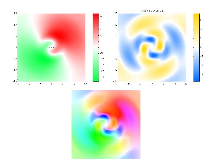
Use of orthogonal color channels to preserve independence of distributions • Period 1 Red-Green • Period 2 Blue-Yellow • The particular color mapping is still not ideal, but all the symmetries are maintained in the final image. Period 1 structure is delineated by R/G boundaries, period 2 structure by B/Y boundaries.

Effects of forcing data into wrong channel Period 1 Purple/Green Period 2 Achromatic Period 1 R/G Period 2 B/Y The image on the left appears fuzzy, as the less-important period 2 behavior is mapped into the high-spatial frequency sensitive achromatic channel. The image is much sharper when mapping the two components directly to color.

Conclusions • This general strategy is applicable when multiple spatially orthogonal channels are presented simultaneously • Data channels should be mapped appropriately – Color vision provides one high-spatial-frequency channel and two similar lower-spatial-frequency channels – Relative importance of data should be considered • Provides a robust strategy in numerous applications