Discretizing The Concentration Equation Mike Grimm Math 1110

Discretizing The Concentration Equation Mike Grimm Math 1110 March 11, 2002 1

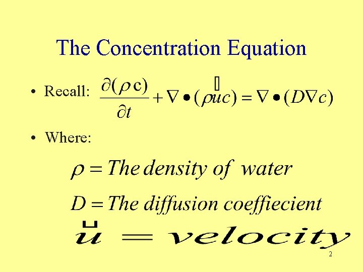
The Concentration Equation • Recall: • Where: 2

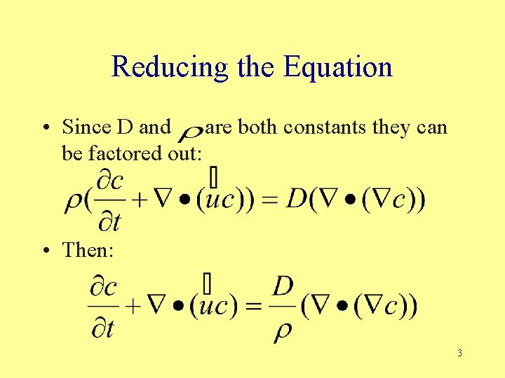
Reducing the Equation • Since D and are both constants they can be factored out: • Then: 3

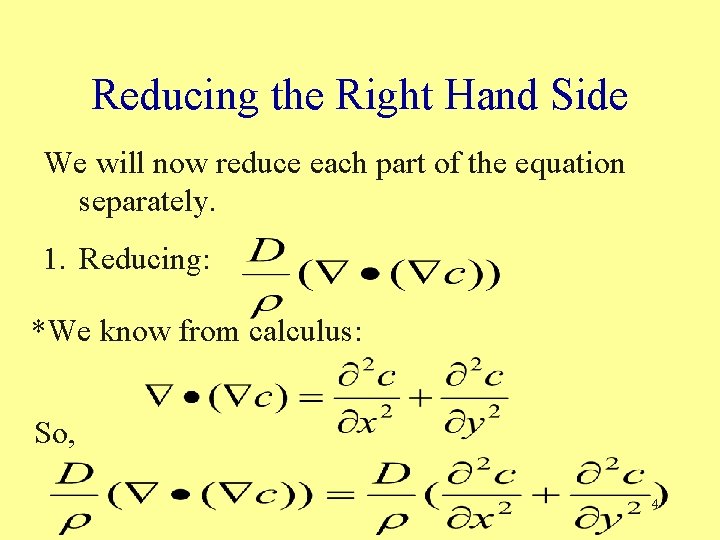
Reducing the Right Hand Side We will now reduce each part of the equation separately. 1. Reducing: *We know from calculus: So, 4

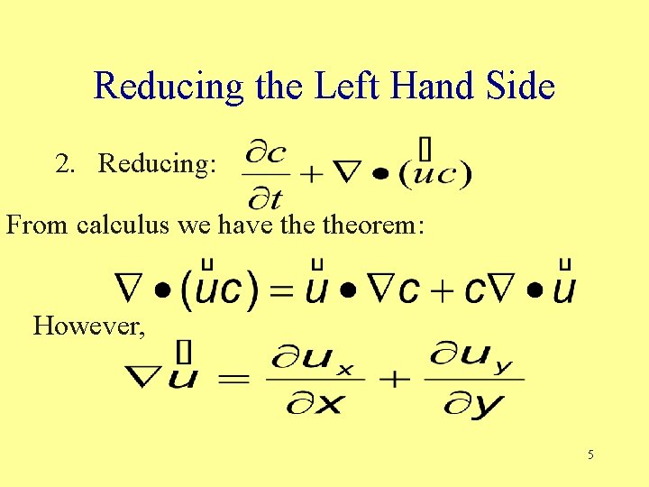
Reducing the Left Hand Side 2. Reducing: From calculus we have theorem: However, 5

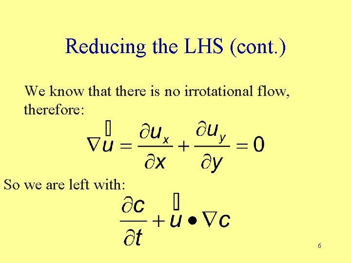
Reducing the LHS (cont. ) We know that there is no irrotational flow, therefore: So we are left with: 6

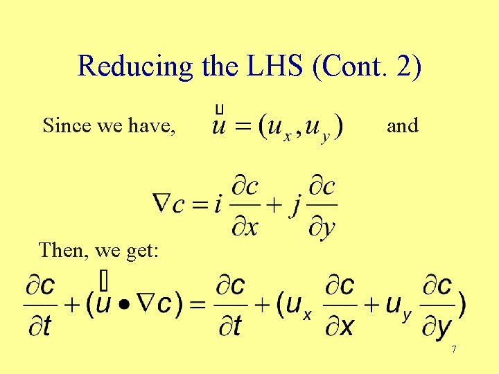
Reducing the LHS (Cont. 2) Since we have, and Then, we get: 7

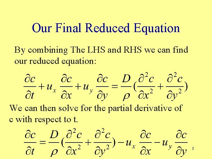
Our Final Reduced Equation By combining The LHS and RHS we can find our reduced equation: We can then solve for the partial derivative of c with respect to t. 8

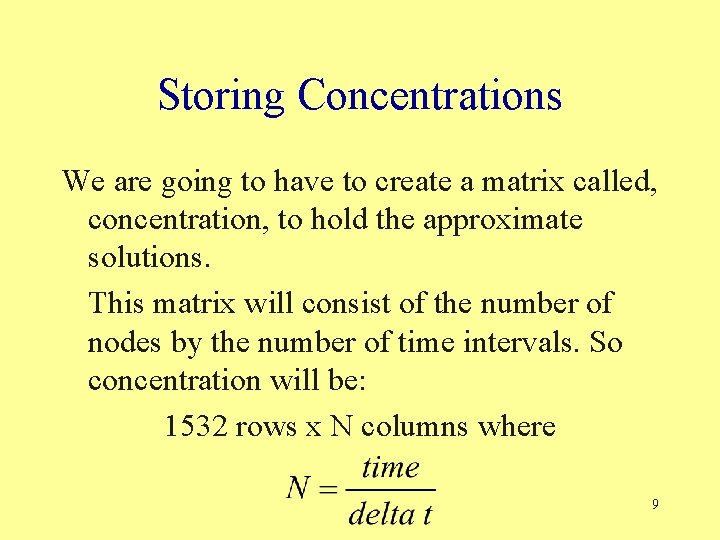
Storing Concentrations We are going to have to create a matrix called, concentration, to hold the approximate solutions. This matrix will consist of the number of nodes by the number of time intervals. So concentration will be: 1532 rows x N columns where 9

Discretizing the Equation • Now that we have the equation for the concentration at a any point and any time, we need to solve that equation. • The Problem: This equation cannot be solved because there an infinite number of positions and infinite times. • What we must do is create an approximation of that solution. 10

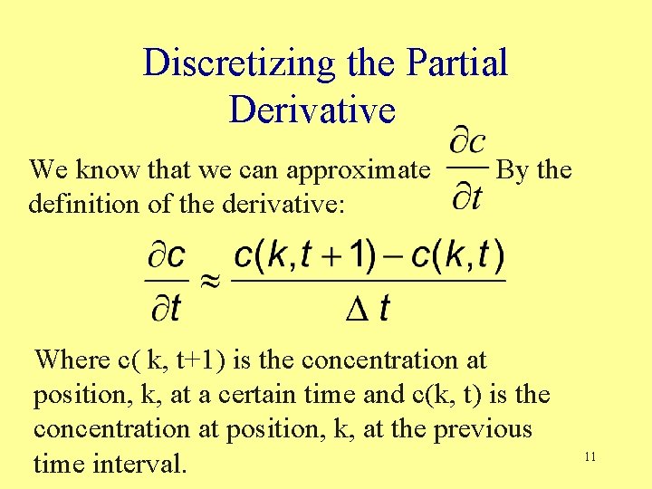
Discretizing the Partial Derivative We know that we can approximate definition of the derivative: By the Where c( k, t+1) is the concentration at position, k, at a certain time and c(k, t) is the concentration at position, k, at the previous time interval. 11

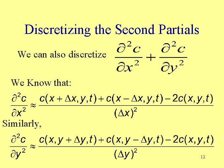
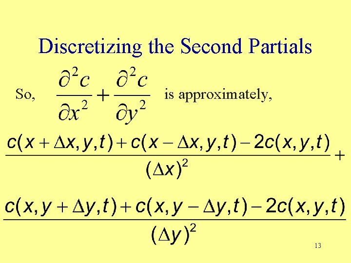
Discretizing the Second Partials We can also discretize We Know that: Similarly, 12

Discretizing the Second Partials So, is approximately, 13

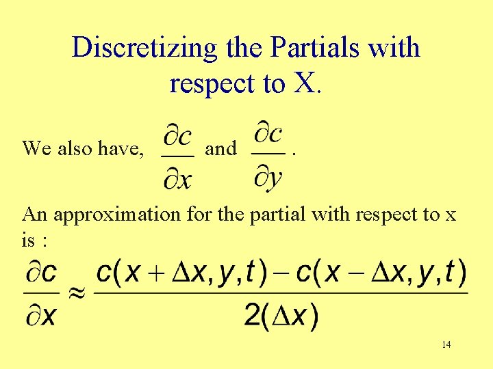
Discretizing the Partials with respect to X. We also have, and . An approximation for the partial with respect to x is : 14

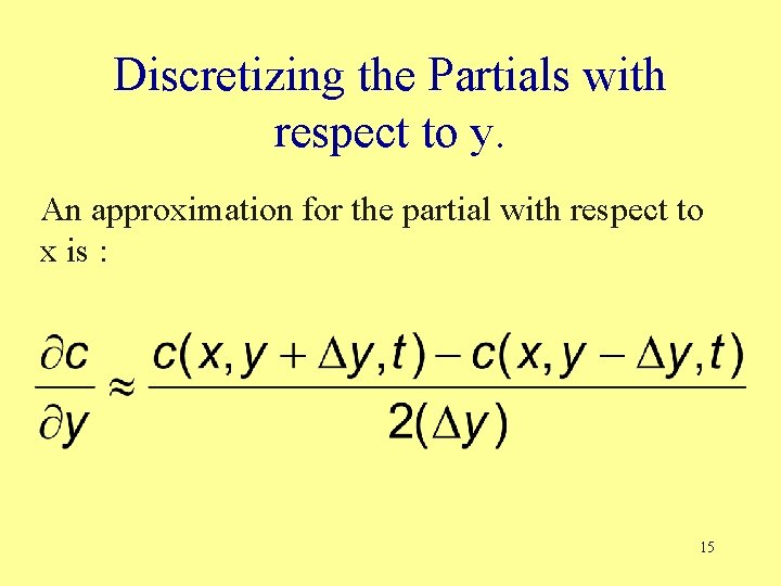
Discretizing the Partials with respect to y. An approximation for the partial with respect to x is : 15

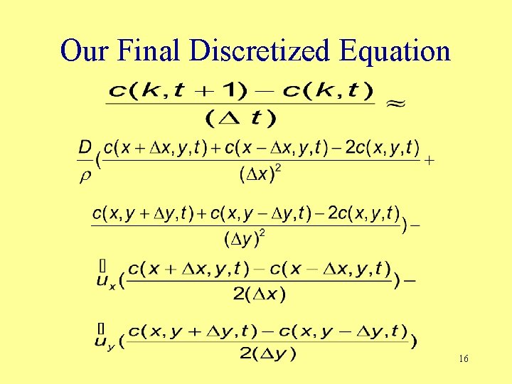
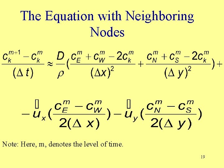
Our Final Discretized Equation 16

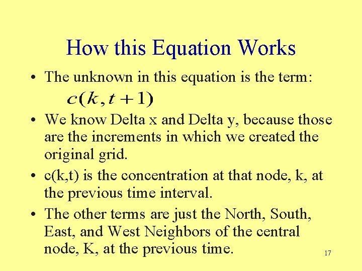
How this Equation Works • The unknown in this equation is the term: • We know Delta x and Delta y, because those are the increments in which we created the original grid. • c(k, t) is the concentration at that node, k, at the previous time interval. • The other terms are just the North, South, East, and West Neighbors of the central node, K, at the previous time. 17

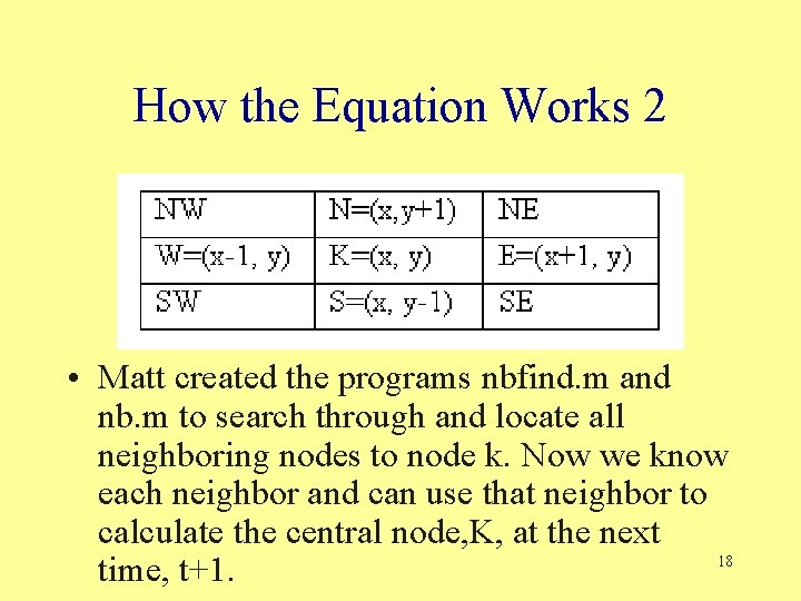
How the Equation Works 2 • Matt created the programs nbfind. m and nb. m to search through and locate all neighboring nodes to node k. Now we know each neighbor and can use that neighbor to calculate the central node, K, at the next 18 time, t+1.

The Equation with Neighboring Nodes Note: Here, m, denotes the level of time. 19

Conditions To approximate the solution we must first have the Initial and boundary conditions. – Initial conditions: c(x, y, 0) = g(x) for all x, y in our domain. Where g(x) is some function to be specified later. – Boundary conditions: c(x, y, t) = 0 for x, y on our boundary at any time, t. 20

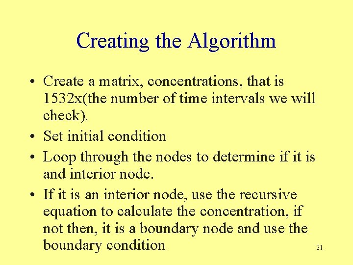
Creating the Algorithm • Create a matrix, concentrations, that is 1532 x(the number of time intervals we will check). • Set initial condition • Loop through the nodes to determine if it is and interior node. • If it is an interior node, use the recursive equation to calculate the concentration, if not then, it is a boundary node and use the 21 boundary condition

22