DiscreteTime State Space Models CSE 421 Digital Control
- Slides: 14

Discrete-Time State Space Models CSE 421 Digital Control Lecture 9 1

Introduction • A physical system is usually modeled by differential equations (i. e. continuous-time). • For digital control, it is required to transform state space models from continuous to discrete-time (i. e. discretization). • Here, we study the conversion of continuous-time state-space into discrete-time with the assumption that the input is constant between samples. • Let us first review the response of a continuous-time system. 2

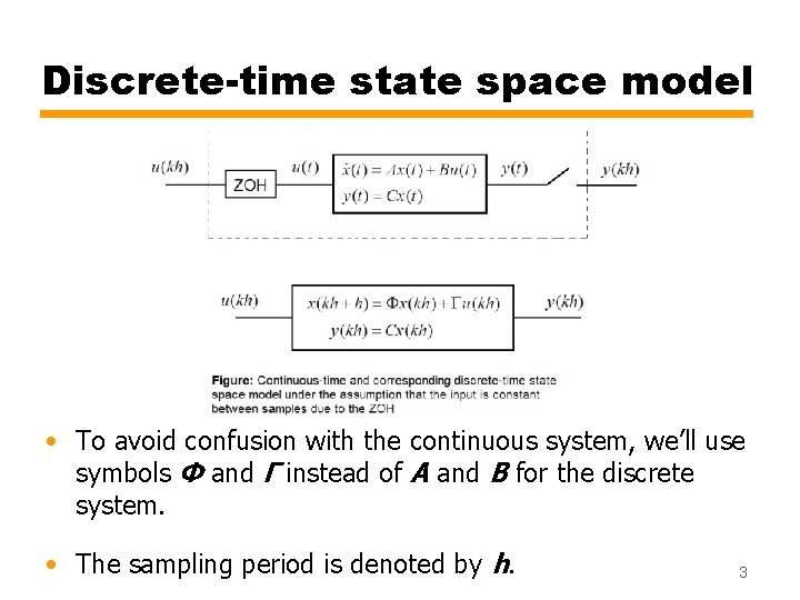
Discrete-time state space model • To avoid confusion with the continuous system, we’ll use symbols Φ and Γ instead of A and B for the discrete system. • The sampling period is denoted by h. 3

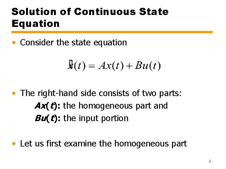
Solution of Continuous State Equation • Consider the state equation • The right-hand side consists of two parts: Ax(t): the homogeneous part and Bu(t): the input portion • Let us first examine the homogeneous part 4

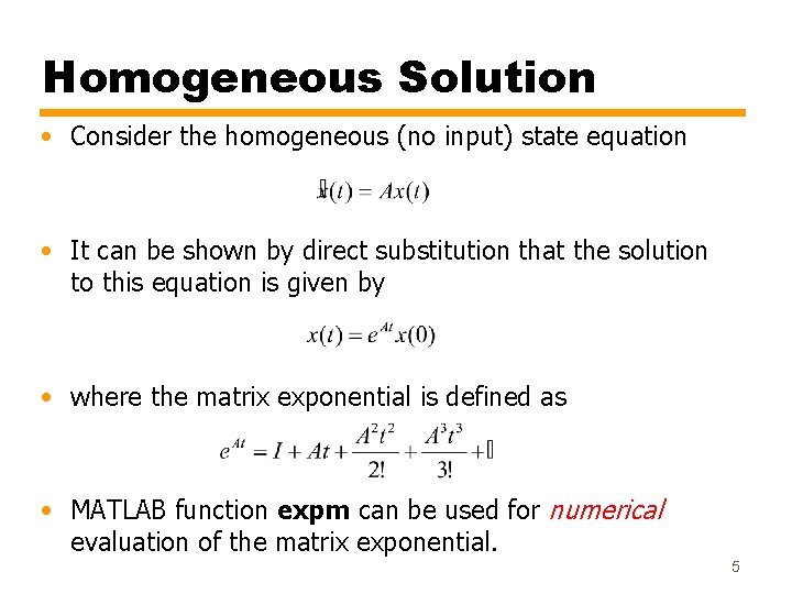
Homogeneous Solution • Consider the homogeneous (no input) state equation • It can be shown by direct substitution that the solution to this equation is given by • where the matrix exponential is defined as • MATLAB function expm can be used for numerical evaluation of the matrix exponential. 5

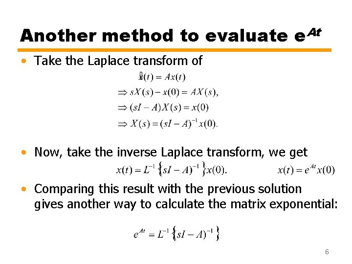
Another method to evaluate e. At • Take the Laplace transform of • Now, take the inverse Laplace transform, we get • Comparing this result with the previous solution gives another way to calculate the matrix exponential: 6

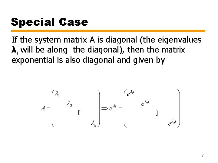
Special Case If the system matrix A is diagonal (the eigenvalues λi will be along the diagonal), then the matrix exponential is also diagonal and given by 7

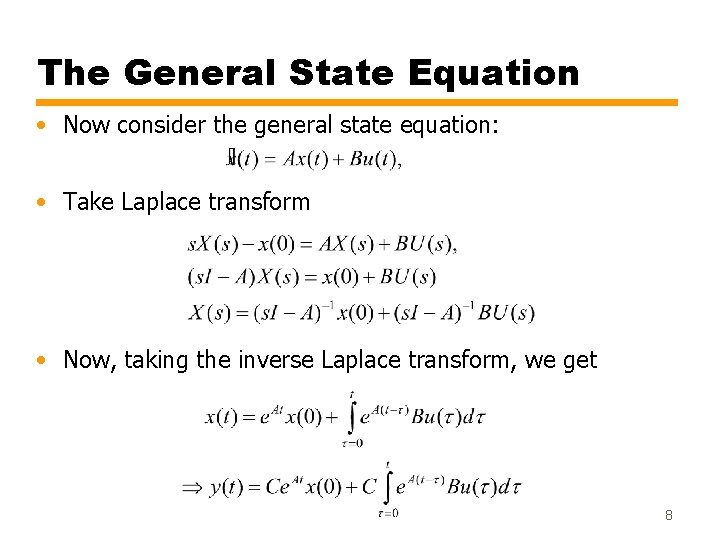
The General State Equation • Now consider the general state equation: • Take Laplace transform • Now, taking the inverse Laplace transform, we get 8

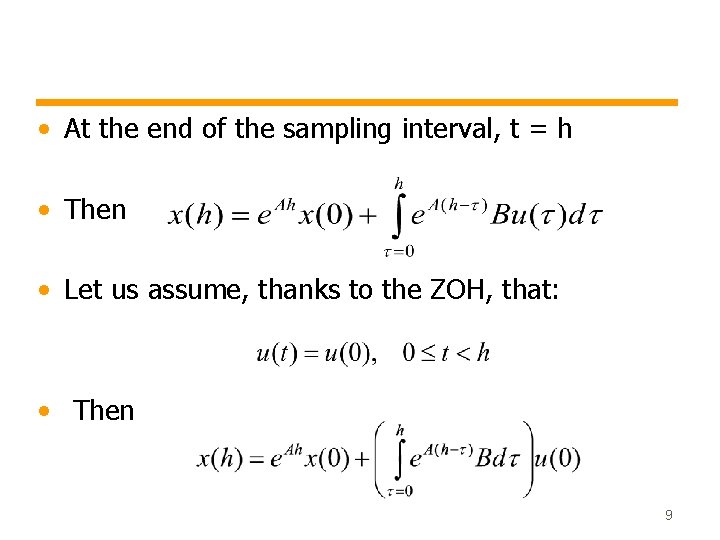
• At the end of the sampling interval, t = h • Then • Let us assume, thanks to the ZOH, that: • Then 9

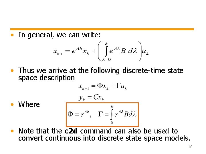
• In general, we can write: • Thus we arrive at the following discrete-time state space description • Where • Note that the c 2 d command can also be used to convert continuous into discrete state space models. 10

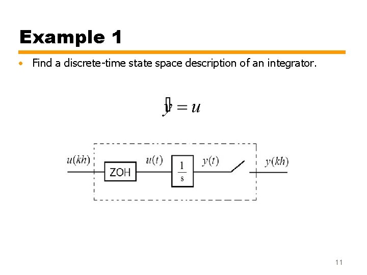
Example 1 • Find a discrete-time state space description of an integrator. 11

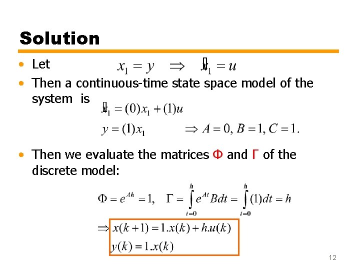
Solution • Let • Then a continuous-time state space model of the system is • Then we evaluate the matrices Φ and Γ of the discrete model: 12

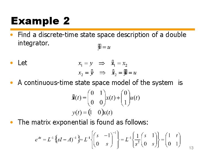
Example 2 • Find a discrete-time state space description of a double integrator. • Let • A continuous-time state space model of the system is • The matrix exponential is found as follows: 13

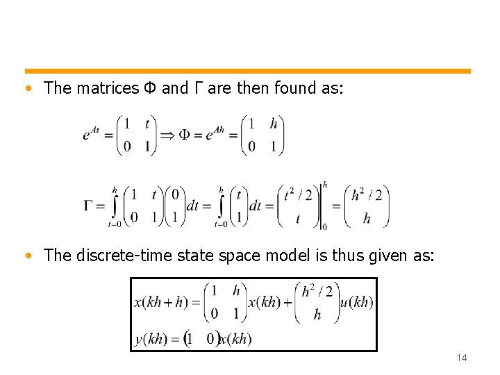
• The matrices Φ and Γ are then found as: • The discrete-time state space model is thus given as: 14