Discrete vortex method Ana Lavern Simavilla M Victoria

Discrete vortex method Ana Laverón Simavilla Mª Victoria Lapuerta González

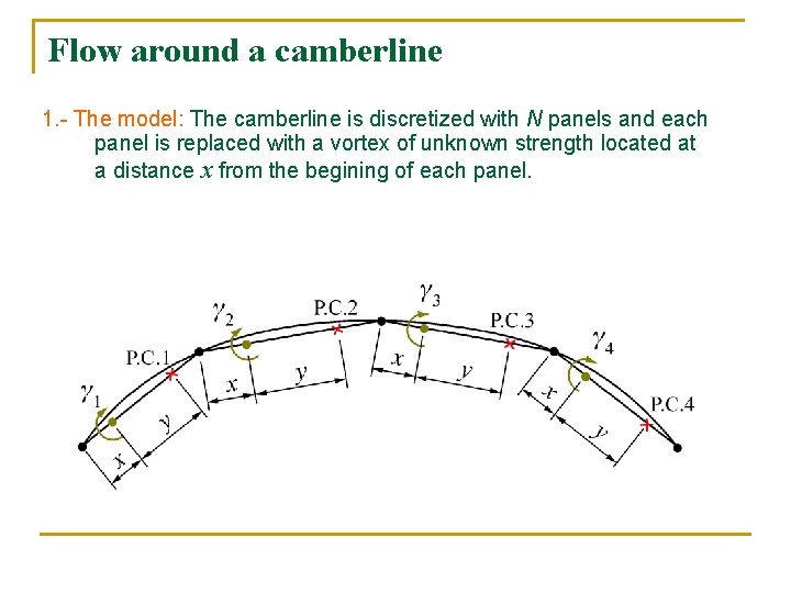
Flow around a camberline 1. - The model: The camberline is discretized with N panels and each panel is replaced with a vortex of unknown strength located at a distance x from the begining of each panel.

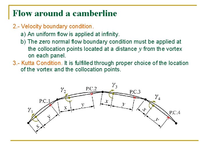
Flow around a camberline 2. - Velocity boundary condition. a) An uniform flow is applied at infinity. b) The zero normal flow boundary condition must be applied at the collocation points located at a distance y from the vortex on each panel. 3. - Kutta Condition. It is fulfilled through proper choice of the location of the vortex and the collocation points.

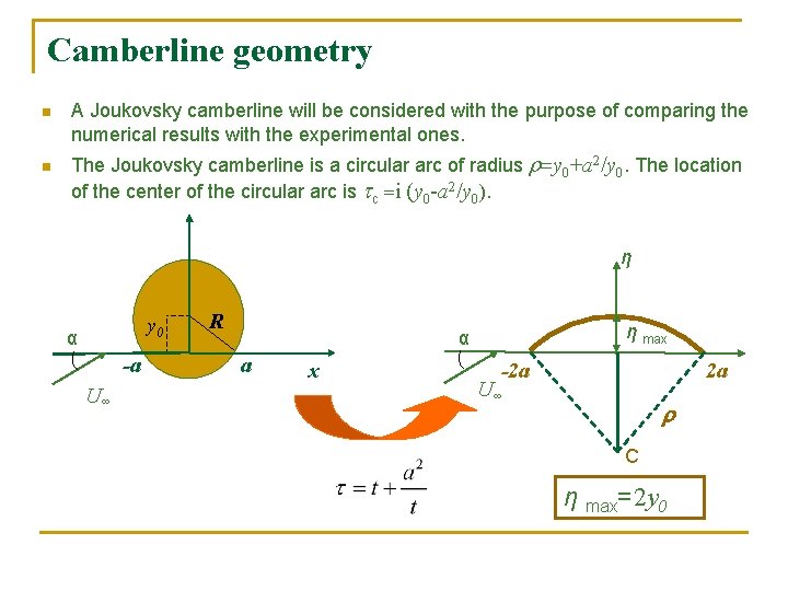
Camberline geometry n n A Joukovsky camberline will be considered with the purpose of comparing the numerical results with the experimental ones. The Joukovsky camberline is a circular arc of radius =y 0+a 2/y 0. The location of the center of the circular arc is tc =i (y 0 -a 2/y 0). η y 0 α -a U∞ R η max α a x -2 a 2 a U∞ r C η max=2 y 0

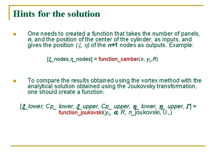
Hints for the solution n One needs to created a function that takes the number of panels, n, and the position of the center of the cylinder, as inputs, and gives the position (x, h) of the n+1 nodes as outputs. Example: [ξ_nodes, η_nodes] = function_camber(n, y 0, R) n To compare the results obtained using the vortex method with the analytical solution obtained using the Joukovsky transformation, one should create a function: [ _lower, Cp_ lower, _upper, Cp_ upper, _ lower, _ upper, ] = function_joukovski(y 0, , R, n_joukovski, U∞)

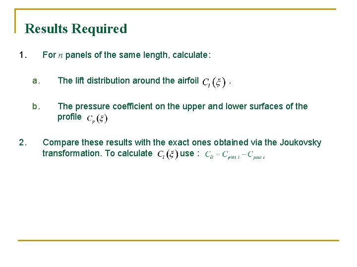
Results Required 1. 2. For n panels of the same length, calculate: a. The lift distribution around the airfoil b. The pressure coefficient on the upper and lower surfaces of the profile . Compare these results with the exact ones obtained via the Joukovsky transformation. To calculate use :

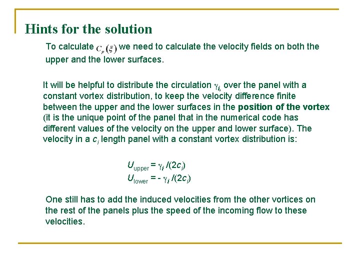
Hints for the solution To calculate we need to calculate the velocity fields on both the upper and the lower surfaces. It will be helpful to distribute the circulation gi, over the panel with a constant vortex distribution, to keep the velocity difference finite between the upper and the lower surfaces in the position of the vortex (it is the unique point of the panel that in the numerical code has different values of the velocity on the upper and lower surface). The velocity in a ci length panel with a constant vortex distribution is: Uupper = gi /(2 ci) Ulower = - gi /(2 ci) One still has to add the induced velocities from the other vortices on the rest of the panels plus the speed of the incoming flow to these velocities.

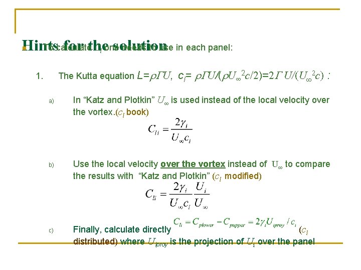
Hints for the solution To calculate C one needs to use in each panel: n l The Kutta equation L= U, 1. a) b) c) cl= U/( U∞ 2 c/2)=2 U/(U∞ 2 c) : In “Katz and Plotkin” U∞ is used instead of the local velocity over the vortex. (cl book) Use the local velocity over the vortex instead of U∞ to compare the results with “Katz and Plotkin” (cl modified) Finally, calculate directly (c l distributed) where Uiproy is the projection of Ui over the panel

Hints for the solution n Take R=1, U∞=1 x and y, leave them as n To analyze the influence of the parameters in the code. n The matlab “diff” function may help you to calculate the increments in the code. n The matlab “spline” function will be helpful to interpolate: Yj=spline(Xi, Yi, Xj) n When numerical Cl y Cp are representing it is assumed that the loads are applied at the position of the vortex.

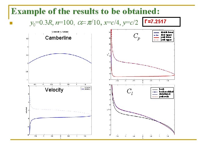
Example of the results to be obtained: n y 0=0. 3 R, n=100, a=p/10, x=c/4, y=c/2 Cp Camberline Velocity Cl Г=7. 2517 distrib lower distr upper jouk lower jouk upper book modified distributed joukovski

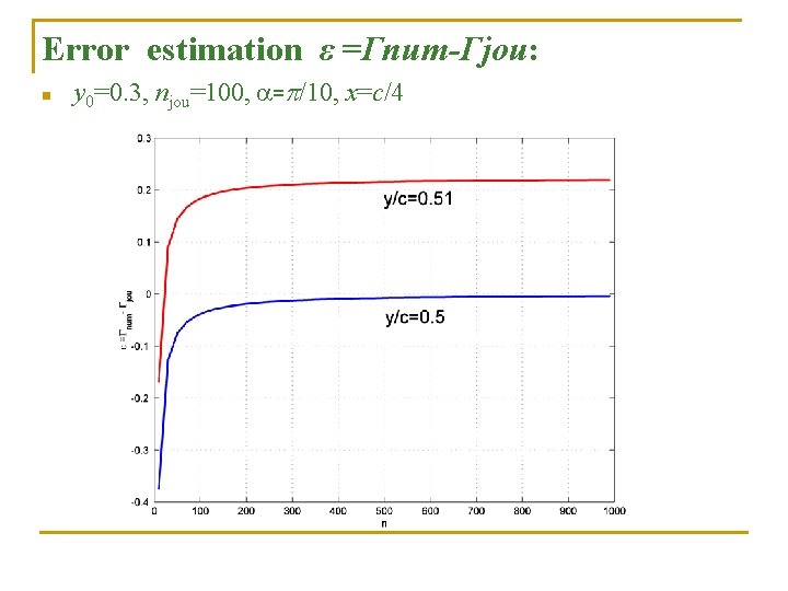
Error estimation ε =Γnum-Γjou: n y 0=0. 3, njou=100, a=p/10, x=c/4