Discrete Optimization Lecture 2 Last Time 1 Course

Discrete Optimization Lecture #2 Last Time 1. Course Overview » » A taxonomy of optimization problems Course introduction, requirements and schedule 2. Some Basics of Optimization » » Local and global optima Feasibility Convex programming 3. Algorithms and Complexity » 2008/2/27 Problems, algorithms, and complexity Shi-Chung Chang, NTUEE, GIIE, GICE 1

Discrete Optimization Lecture #2 Last Time: Reading Assignments 1. Chapter 1 and the Appendix of [Pa. S 82] 2. Chapter 1 of [Ga. J 79] [Pa. S 82] C. H. Papadimitriou, K. Steiglitz, Combinatorial Optimization: Algorithms and Complexity, Prentice Hall, 1982. [Ga. J 79] M. R. Garey and D. S. Johnson, Computers and Intractability: A Guide to the Theory of NP-Completeness , Series of Books in the Mathematical Sciences, 1979. 2008/2/27 Shi-Chung Chang, NTUEE, GIIE, GICE 2

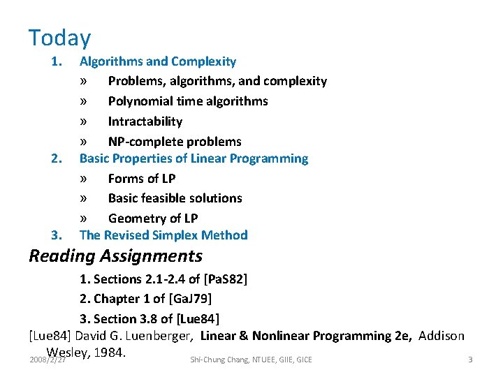
Today 1. 2. 3. Algorithms and Complexity » Problems, algorithms, and complexity » Polynomial time algorithms » Intractability » NP-complete problems Basic Properties of Linear Programming » Forms of LP » Basic feasible solutions » Geometry of LP The Revised Simplex Method Reading Assignments 1. Sections 2. 1 -2. 4 of [Pa. S 82] 2. Chapter 1 of [Ga. J 79] 3. Section 3. 8 of [Lue 84] David G. Luenberger, Linear & Nonlinear Programming 2 e, Addison Wesley, 1984. 2008/2/27 Shi-Chung Chang, NTUEE, GIIE, GICE 3

§ 1. 4 Algorithms and complexity For a given (optimization) problem, Questions: 1) how hard is the problem. 2) does there exist an efficient solution algorithm? è Computational complexity analysis (a worst case analysis) 2008/2/27 Shi-Chung Chang, NTUEE, GIIE, GICE 4

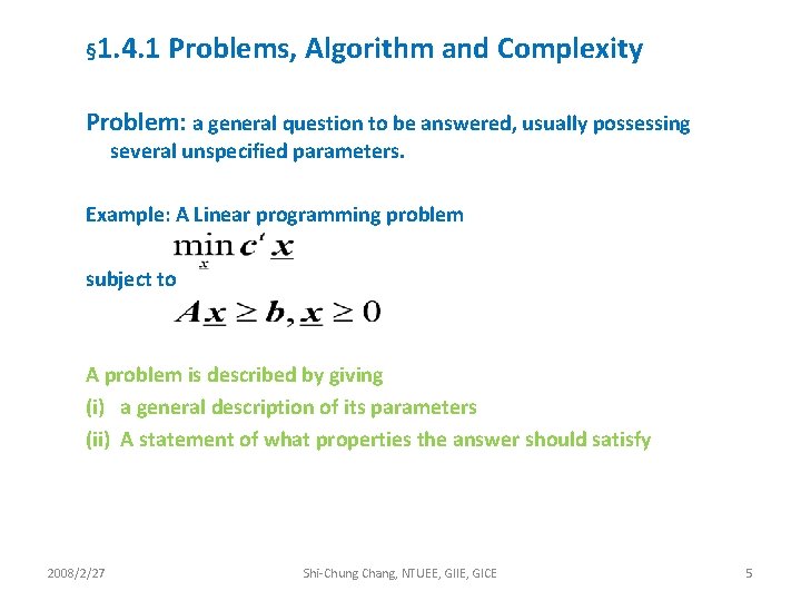
§ 1. 4. 1 Problems, Algorithm and Complexity Problem: a general question to be answered, usually possessing several unspecified parameters. Example: A Linear programming problem subject to A problem is described by giving (i) a general description of its parameters (ii) A statement of what properties the answer should satisfy 2008/2/27 Shi-Chung Chang, NTUEE, GIIE, GICE 5

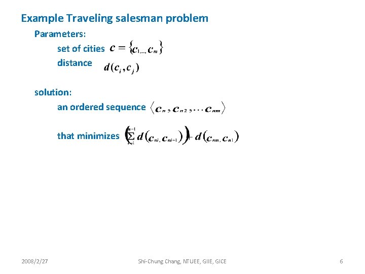
Example Traveling salesman problem Parameters: set of cities distance solution: an ordered sequence that minimizes 2008/2/27 Shi-Chung Chang, NTUEE, GIIE, GICE 6

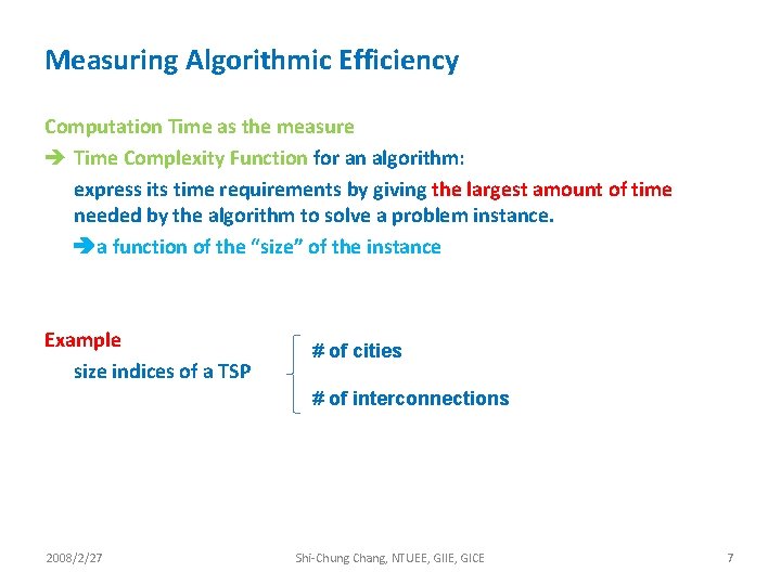
Measuring Algorithmic Efficiency Computation Time as the measure è Time Complexity Function for an algorithm: express its time requirements by giving the largest amount of time needed by the algorithm to solve a problem instance. a function of the “size” of the instance Example size indices of a TSP # of cities # of interconnections 2008/2/27 Shi-Chung Chang, NTUEE, GIIE, GICE 7

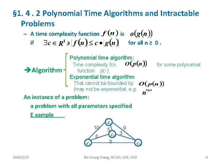
§ 1. 4. 2 Polynomial Time Algorithms and Intractable Problems – A time complexity function if is for all n ≥ 0. Polynomial time algorithm: èAlgorithm Time complexity fcn. function p(･). for some polynomial Exponential time algorithm That cannot be bounded by (may not be exponential, e. g. An instance of a problem: a problem with all parameters specified E xample 10 6 2008/2/27 5 3 9 8 Shi-Chung Chang, NTUEE, GIIE, GICE 8

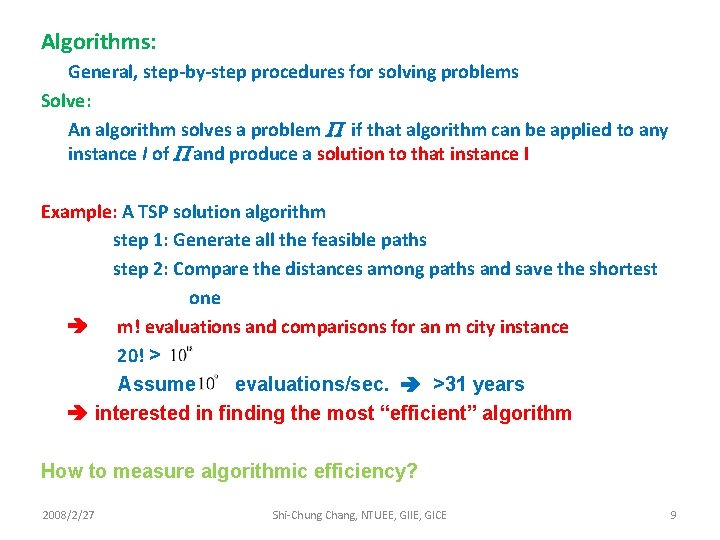
Algorithms: General, step-by-step procedures for solving problems Solve: An algorithm solves a problem P if that algorithm can be applied to any instance I of P and produce a solution to that instance I Example: A TSP solution algorithm step 1: Generate all the feasible paths step 2: Compare the distances among paths and save the shortest one m! evaluations and comparisons for an m city instance 20! > Assume evaluations/sec. >31 years interested in finding the most “efficient” algorithm How to measure algorithmic efficiency? 2008/2/27 Shi-Chung Chang, NTUEE, GIIE, GICE 9

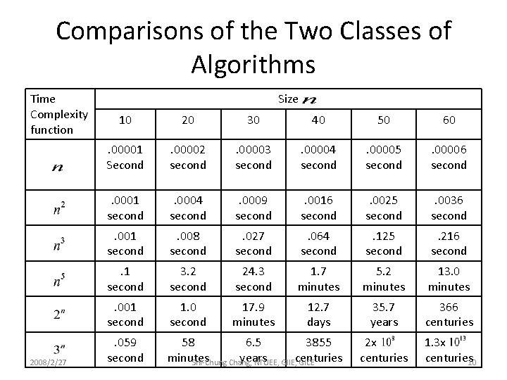
Comparisons of the Two Classes of Algorithms Time Complexity function 2008/2/27 Size 10 20 30 40 50 60 . 00001 Second . 00002 second . 00003 second . 00004 second . 00005 second . 00006 second . 0001 second . 0004 second . 0009 second . 0016 second . 0025 second . 0036 second . 001 second . 008 second . 027 second . 064 second . 125 second . 216 second . 1 second 3. 2 second 24. 3 second 1. 7 minutes 5. 2 minutes 13. 0 minutes . 001 second 1. 0 second 17. 9 minutes 12. 7 days 35. 7 years 366 centuries . 059 second 58 6. 5 3855 minutes years Shi-Chung Chang, NTUEE, GIIE, centuries GICE 2 x centuries 1. 3 x centuries 10

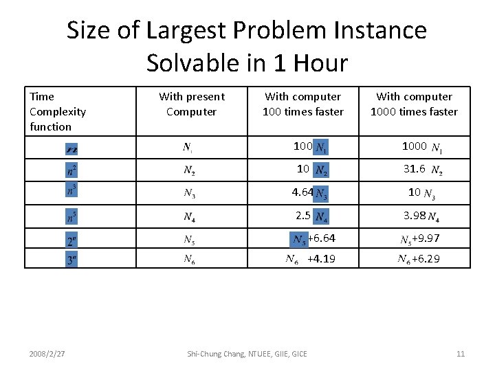
Size of Largest Problem Instance Solvable in 1 Hour Time Complexity function 2008/2/27 With present Computer With computer 100 times faster With computer 1000 times faster 1000 10 31. 6 4. 64 10 2. 5 3. 98 +6. 64 +9. 97 +4. 19 +6. 29 Shi-Chung Chang, NTUEE, GIIE, GICE 11

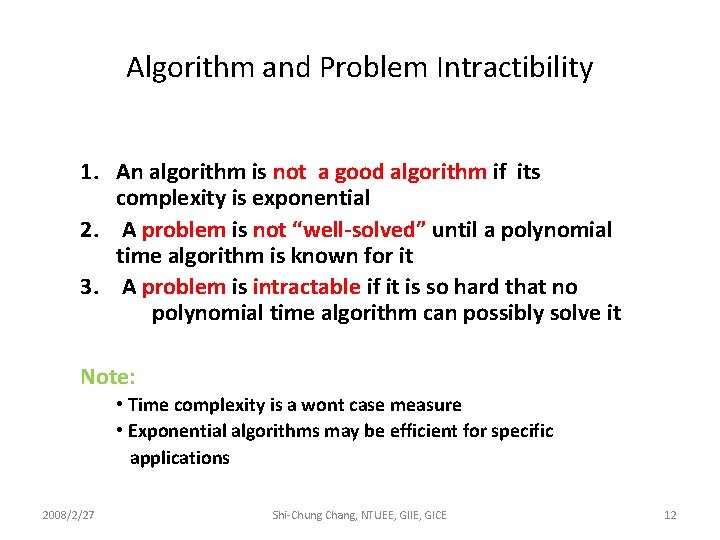
Algorithm and Problem Intractibility 1. An algorithm is not a good algorithm if its complexity is exponential 2. A problem is not “well-solved” until a polynomial time algorithm is known for it 3. A problem is intractable if it is so hard that no polynomial time algorithm can possibly solve it Note: • Time complexity is a wont case measure • Exponential algorithms may be efficient for specific applications 2008/2/27 Shi-Chung Chang, NTUEE, GIIE, GICE 12

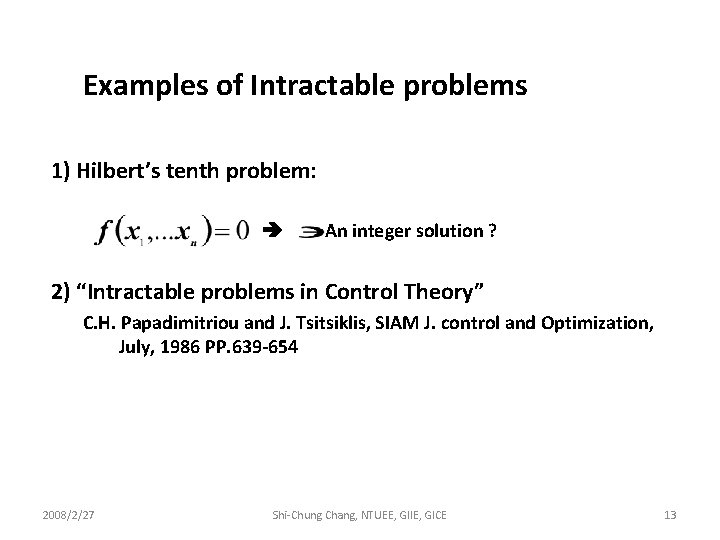
Examples of Intractable problems 1) Hilbert’s tenth problem: An integer solution ? 2) “Intractable problems in Control Theory” C. H. Papadimitriou and J. Tsitsiklis, SIAM J. control and Optimization, July, 1986 PP. 639 -654 2008/2/27 Shi-Chung Chang, NTUEE, GIIE, GICE 13

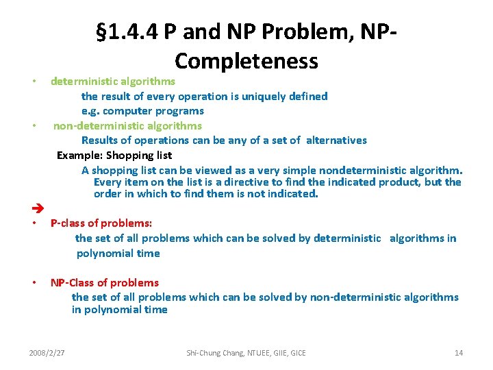
• • § 1. 4. 4 P and NP Problem, NPCompleteness deterministic algorithms the result of every operation is uniquely defined e. g. computer programs non-deterministic algorithms Results of operations can be any of a set of alternatives Example: Shopping list A shopping list can be viewed as a very simple nondeterministic algorithm. Every item on the list is a directive to find the indicated product, but the order in which to find them is not indicated. • P-class of problems: the set of all problems which can be solved by deterministic algorithms in polynomial time • NP-Class of problems the set of all problems which can be solved by non-deterministic algorithms in polynomial time 2008/2/27 Shi-Chung Chang, NTUEE, GIIE, GICE 14

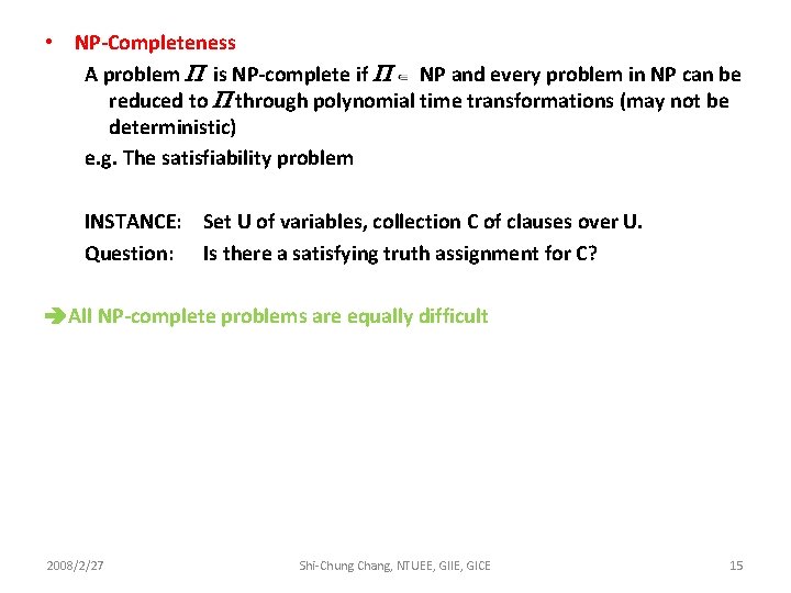
• NP-Completeness A problem P is NP-complete if P NP and every problem in NP can be reduced to P through polynomial time transformations (may not be deterministic) e. g. The satisfiability problem INSTANCE: Set U of variables, collection C of clauses over U. Question: Is there a satisfying truth assignment for C? All NP-complete problems are equally difficult 2008/2/27 Shi-Chung Chang, NTUEE, GIIE, GICE 15

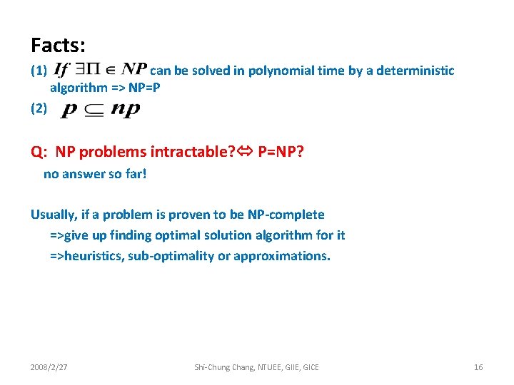
Facts: (1) can be solved in polynomial time by a deterministic algorithm => NP=P (2) Q: NP problems intractable? P=NP? no answer so far! Usually, if a problem is proven to be NP-complete =>give up finding optimal solution algorithm for it =>heuristics, sub-optimality or approximations. 2008/2/27 Shi-Chung Chang, NTUEE, GIIE, GICE 16

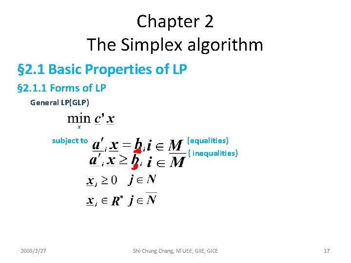
Chapter 2 The Simplex algorithm § 2. 1 Basic Properties of LP § 2. 1. 1 Forms of LP General LP(GLP) subject to 2008/2/27 (equalities) ( inequalities) Shi-Chung Chang, NTUEE, GIIE, GICE 17

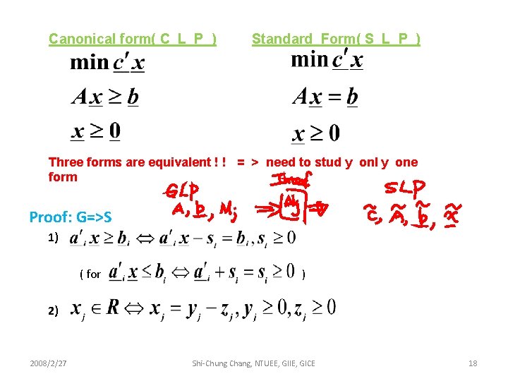
Canonical form( C L P ) Standard Form( S L P ) Three forms are equivalent ! ! = > need to stud y onl y one form Proof: G=>S 1) ( for ) 2) 2008/2/27 Shi-Chung Chang, NTUEE, GIIE, GICE 18

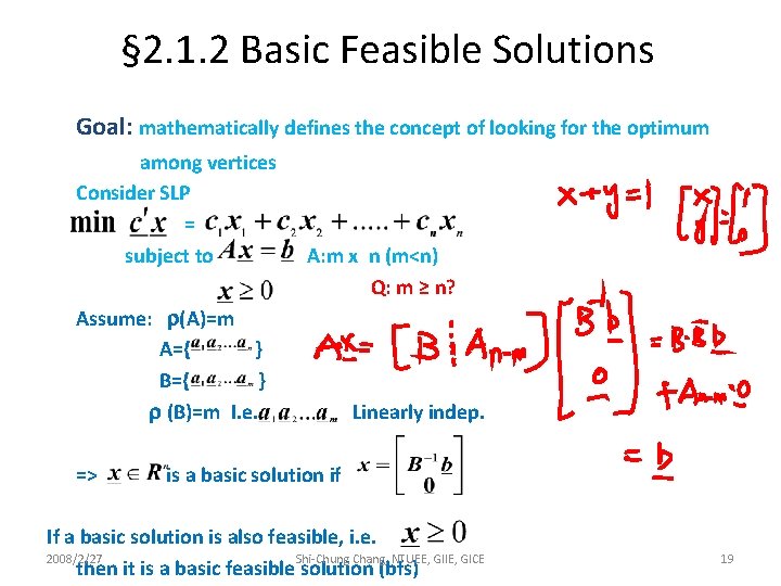
§ 2. 1. 2 Basic Feasible Solutions Goal: mathematically defines the concept of looking for the optimum among vertices Consider SLP = subject to A: m x n (m<n) Q: m ≥ n? Assume: r(A)=m A={ } B={ } r (B)=m I. e. => Linearly indep. is a basic solution if If a basic solution is also feasible, i. e. 2008/2/27 Shi-Chung Chang, NTUEE, GIIE, GICE then it is a basic feasible solution (bfs) 19

Example min[0 2 0 1 0 0 5] subject to B ① and = a bfs ② B= 2008/2/27 => Shi-Chung Chang, NTUEE, GIIE, GICE basic not feasible 20

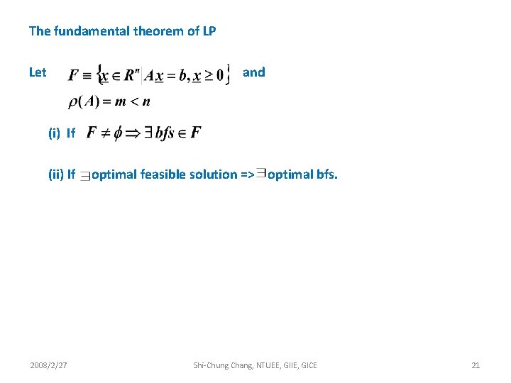
The fundamental theorem of LP Let and (i) If (ii) If 2008/2/27 optimal feasible solution => optimal bfs. Shi-Chung Chang, NTUEE, GIIE, GICE 21

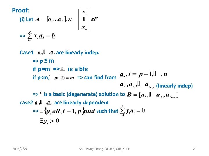
Proof: (i) Let => Case 1 are linearly indep. => p ≤ m if p=m => is a bfs if p<m, => can find from (linearly indep) => is a basic (degenerate) solution to case 2 are linearly dependent => such that 2008/2/27 Shi-Chung Chang, NTUEE, GIIE, GICE 22

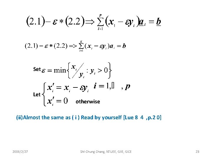
Set Let otherwise (ii)Almost the same as ( i ) Read by yourself [Lue 8 4 , p. 2 0] 2008/2/27 Shi-Chung Chang, NTUEE, GIIE, GICE 23

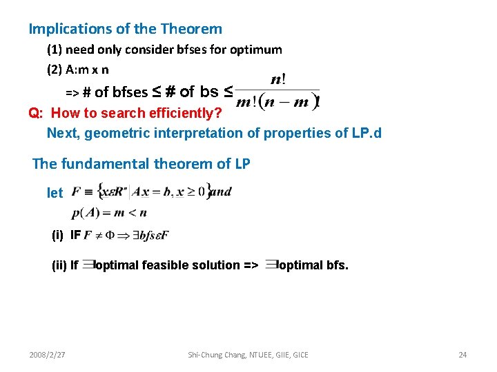
Implications of the Theorem (1) need only consider bfses for optimum (2) A: m x n => # of bfses ≤ # of bs ≤ Q: How to search efficiently? Next, geometric interpretation of properties of LP. d The fundamental theorem of LP let (i) IF (ii) If 2008/2/27 optimal feasible solution => optimal bfs. Shi-Chung Chang, NTUEE, GIIE, GICE 24

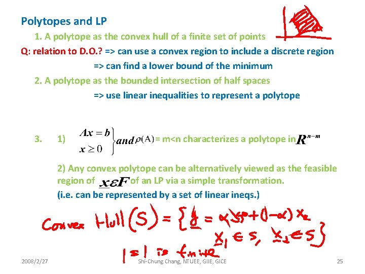
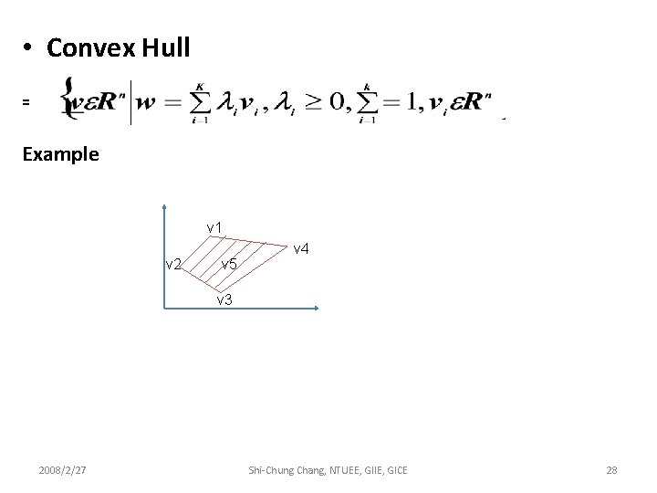
Polytopes and LP 1. A polytope as the convex hull of a finite set of points Q: relation to D. O. ? => can use a convex region to include a discrete region => can find a lower bound of the minimum 2. A polytope as the bounded intersection of half spaces => use linear inequalities to represent a polytope 3. 1) = m<n characterizes a polytope in 2) Any convex polytope can be alternatively viewed as the feasible region of of an LP via a simple transformation. (i. e. can be represented by a set of linear ineqs. ) 2008/2/27 Shi-Chung Chang, NTUEE, GIIE, GICE 25

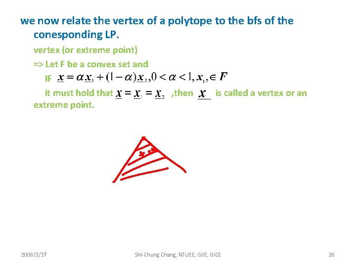
we now relate the vertex of a polytope to the bfs of the conesponding LP. vertex (or extreme point) => Let F be a convex set and IF it must hold that extreme point. 2008/2/27 , then is called a vertex or an Shi-Chung Chang, NTUEE, GIIE, GICE 26

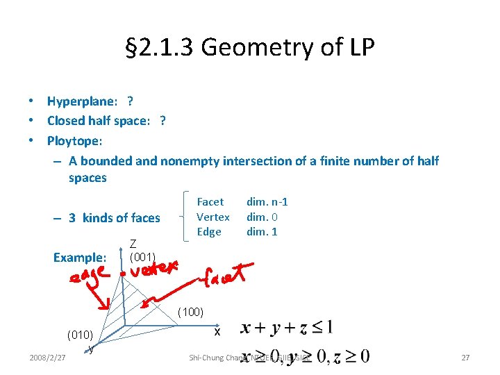
§ 2. 1. 3 Geometry of LP • Hyperplane: ? • Closed half space: ? • Ploytope: – A bounded and nonempty intersection of a finite number of half spaces – 3 kinds of faces Example: Z (001) Facet Vertex Edge dim. n-1 dim. 0 dim. 1 (100) 2008/2/27 (010) y x Shi-Chung Chang, NTUEE, GIIE, GICE 27

• Convex Hull = Example v 1 v 2 v 5 v 4 v 3 2008/2/27 Shi-Chung Chang, NTUEE, GIIE, GICE 28

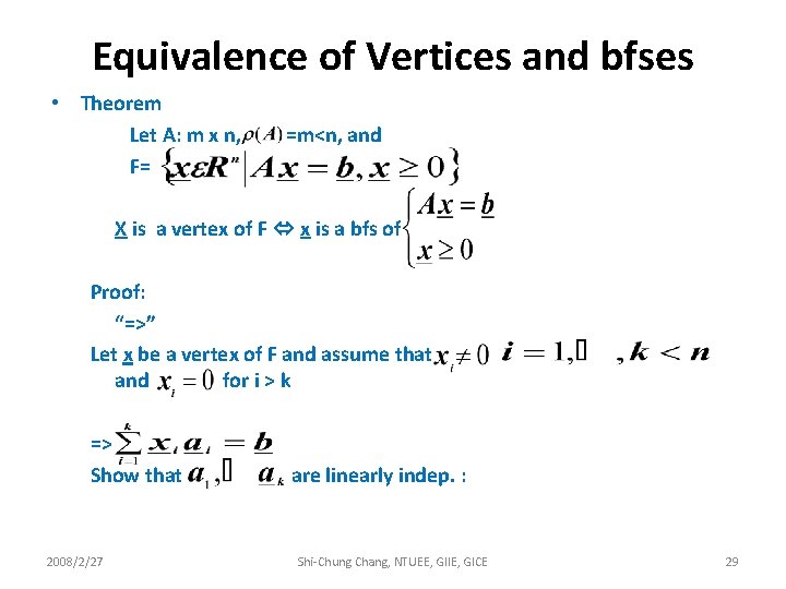
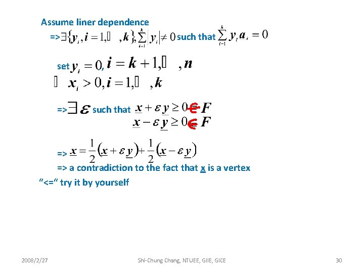
Equivalence of Vertices and bfses • Theorem Let A: m x n, F= =m<n, and X is a vertex of F x is a bfs of Proof: “=>” Let x be a vertex of F and assume that and for i > k => Show that 2008/2/27 are linearly indep. : Shi-Chung Chang, NTUEE, GIIE, GICE 29

Assume liner dependence => set => such that , such that => => a contradiction to the fact that x is a vertex “<=“ try it by yourself 2008/2/27 Shi-Chung Chang, NTUEE, GIIE, GICE 30

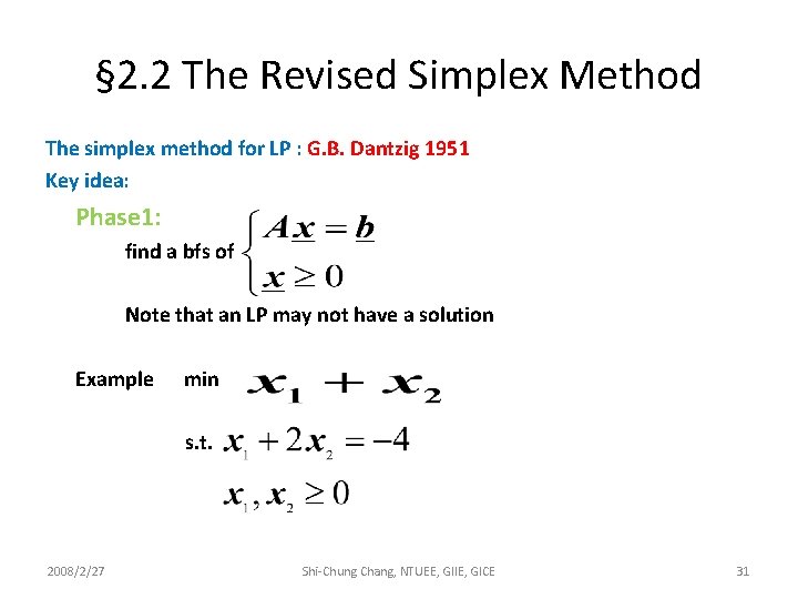
§ 2. 2 The Revised Simplex Method The simplex method for LP : G. B. Dantzig 1951 Key idea: Phase 1: find a bfs of Note that an LP may not have a solution Example min s. t. 2008/2/27 Shi-Chung Chang, NTUEE, GIIE, GICE 31

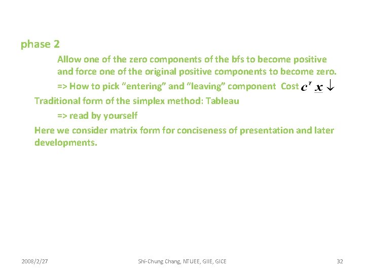
phase 2 Allow one of the zero components of the bfs to become positive and force one of the original positive components to become zero. => How to pick “entering” and “leaving” component Cost Traditional form of the simplex method: Tableau => read by yourself Here we consider matrix form for conciseness of presentation and later developments. 2008/2/27 Shi-Chung Chang, NTUEE, GIIE, GICE 32

SLP: s. t. Assume P(A)=m. Partition A=[B: D] B: m linearly indep. cols. ) Columns of A(Assume the first m (SLP) subject to 2008/2/27 Shi-Chung Chang, NTUEE, GIIE, GICE 33

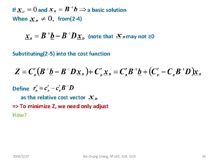
If When and a basic solution from(2 -4) (note that may not ≥ 0 Substituting(2 -5) into the cost function Define as the relative cost vector => To minimize Z, we need only adjust How? 2008/2/27 Shi-Chung Chang, NTUEE, GIIE, GICE 34