Discrete Math Modeling with Biological Applications Math 214

Discrete Math Modeling with Biological Applications Math 214: Unit 2 – Matrix Modeling

Changing Landscape A motivating example

Image of Amazon Park in Eugene, OR Different Types of Landscapes: • • Farmland Forest Industrial Residential

Image of Amazon Park in Eugene, OR Different Types of Landscapes: • • Farmland Forest Industrial Residential

Image of Amazon Park in Eugene, OR Different Types of Landscapes: • • Farmland Forest Industrial Residential

Different Types of Landscapes: • • Farmland Forest Industrial Residential Years (L to R, starting top L): 1936, 1951, 1960, 1968, 1995, 2009

1936 ___ / 10 Farmland ___ / 10 Forest ___ / 10 Industrial ___ / 10 Residential

1951 ___ / 10 Farmland ___ / 10 Forest ___ / 10 Industrial ___ / 10 Residential

1960 ___ / 10 Farmland ___ / 10 Forest ___ / 10 Industrial ___ / 10 Residential

1968 ___ / 10 Farmland ___ / 10 Forest ___ / 10 Industrial ___ / 10 Residential

1995 ___ / 10 Farmland ___ / 10 Forest ___ / 10 Industrial ___ / 10 Residential

2009 ___ / 10 Farmland ___ / 10 Forest ___ / 10 Industrial ___ / 10 Residential

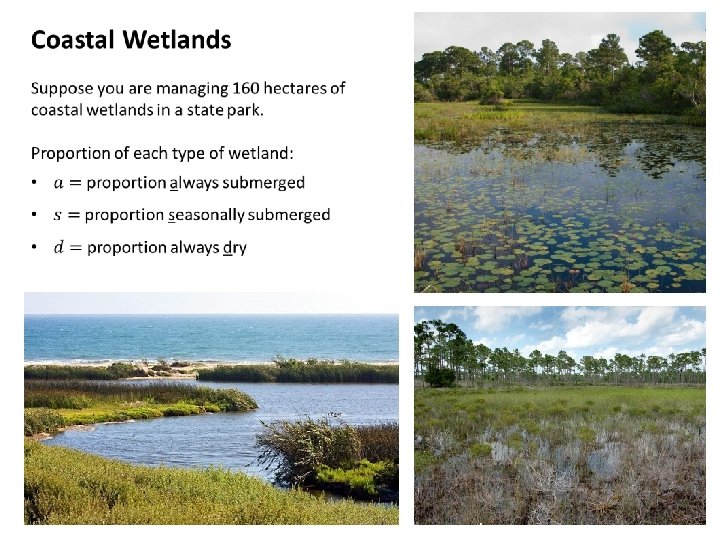
Wetlands are nature’s water filter. Coastal wetlands also help protect land from stormrelated coastal flooding, provide vital habitat for many species of birds, fish, and other wildlife, provide breeding habitat for commercially valuable fish and shellfish, and support recreational activities like hunting, fishing, and birdwatching.

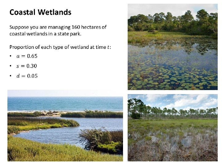
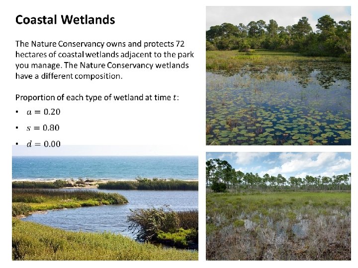
Coastal Wetlands Suppose you are managing 160 hectares of coastal wetlands which are protected as a state park. Classification of wetlands into three land types: • Always submerged • Seasonally submerged • Always dry

Ecological Succession The composition of a particular landscape will change over time. A depiction of primary ecological succession over hundreds of years. Note, biodiversity increases as ecological succession progresses.

Aquatic Succession The composition of a particular landscape will change over time. The image to the right shows aquatic succession. In the top image, the ground beneath the lake is always submerged. As time progresses and more sediment collects in the lake, the lake becomes shallower and the outer edges which used to be seasonally submerged are now always dry land. Eventually, the entire lake is filled in with sediment, and where the lake used to be is now dry land. Note, in this case, biodiversity does not necessarily increase, but the species composition living within the landscape will change.

Constructing Matrix Models A Few Examples

Aquatic Succession Suppose we are looking at a total of 100 hectares of coastal wetlands which is initially always submerge. Every 10 years • 5% of submerged wetlands becomes seasonally submerged • 12% of seasonally submerge wetlands become always dry. • All hectares that are dry remain dry.

Aquatic Succession Suppose we are looking at a total of 100 hectares of coastal wetlands which is initially always submerge. Every 10 years • 5% of submerged wetlands becomes seasonally submerged • 12% of seasonally submerge wetlands become always dry. • All hectares that are dry remain dry.

Aquatic Succession Now suppose the dynamics are more complicated. Every 10 years • 5% of submerged wetlands becomes seasonally submerged • 2% of the seasonally submerged revert back to being always submerged • 12% of seasonally submerge wetlands become always dry • 6% of the always dry land reverts back to being seasonally submerged • 1% of submerged wetlands becomes always dry • 1% of always dry lands become always submerged

Aquatic Succession Littoral Zone contains plants that are completely submerged Emergent Zone contains plants that are partially submerged Riparian Zone contains plants which are not typically submerged but may become submerged when water levels are high Upland Zone contains plants that are never submerged Example of vegetative zones along the shoreline of a freshwater lake, natural pond, storm water pond, or estuary.

Aquatic Succession

Epidemic Dynamics Each day • 4% of the dorm residents became infected with the cold • 20% recovered from their cold and became susceptible again If recovery provides immunity for 1 year, how can the model be modified to account for this?

Matrix Algebra

Matrix Addition Matrix Scalar Multiplication Matrix Subtraction

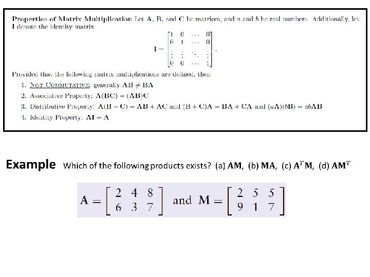
Example

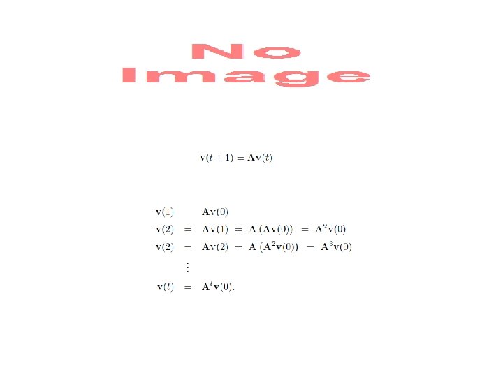
Close-form Solution & Matrix Multiplication

Matrix Multiplication

Matrix Multiplication

Transpose of a Matrix If you take the transpose of a matrix, each row becomes a column, and each column becomes a row. Specifically, row 1 becomes column 1, row 2 becomes column 2, etc.

Long-term Dynamics & Equilibrium Structure A Few Examples

Epidemic Dynamics

Long-term Dynamics

Aquatic Succession

Long-term Dynamics

Aquatic Succession

Aquatic Succession

Leslie Matrix Models
 Egg b) Nymph – not winged c)")
Locusts have three distinct life stages a) Egg b) Nymph – not winged c) Adult – winged • Not all eggs will survive to become adults • Females can only reproduce (lay eggs) during the adult stage of their life Survival Rates (per year) • 2% of eggs survive to become nymphs • 5% of nymphs survive to become adults • 0% of adults survive to the next year i. e. , all adults die shortly after reproduction Fecundity • On average, each adult female will produce 2000 eggs before she dies • Sex ratio of laid eggs is 1: 1
 • 2% of eggs survive to become nymphs •")
Locusts Survival Rates (per year) • 2% of eggs survive to become nymphs • 5% of nymphs survive to become adults • 0% of adults survive to the next year i. e. , all adults die shortly after reproduction Fecundity • On average, each adult female will produce 2000 eggs before she dies • Sex ratio of laid eggs is 1: 1

Leslie Matrix Model

American Bison


Long-term Dynamics & Equilibrium Structure A Few Examples

Long-term Dynamics

Epidemic Dynamics

Aquatic Succession

Aquatic Succession

Aquatic Succession

Leslie Matrix Models
 Egg b) Nymph – not winged c)")
Locusts have three distinct life stages a) Egg b) Nymph – not winged c) Adult – winged • Not all eggs will survive to become adults • Females can only reproduce (lay eggs) during the adult stage of their life Survival Rates (per year) • 2% of eggs survive to become nymphs • 5% of nymphs survive to become adults • 0% of adults survive to the next year i. e. , all adults die shortly after reproduction Fecundity • On average, each adult female will produce 2000 eggs before she dies • Sex ratio of laid eggs is 1: 1
 • 2% of eggs survive to become nymphs •")
Locusts Survival Rates (per year) • 2% of eggs survive to become nymphs • 5% of nymphs survive to become adults • 0% of adults survive to the next year i. e. , all adults die shortly after reproduction Fecundity • On average, each adult female will produce 2000 eggs before she dies • Sex ratio of laid eggs is 1: 1
 • 2% of eggs survive to become nymphs •")
Locusts Survival Rates (per year) • 2% of eggs survive to become nymphs • 5% of nymphs survive to become adults • 0% of adults survive to the next year i. e. , all adults die shortly after reproduction

Leslie Matrix Model

American Bison


Matlab: Finding the roots of a Polynomial


Other Examples

Modifying the Leslie Matrix If the time spent in each size class is not uniform, then some proportion of individuals may need to remain in certain size classes at each time step. This modified matrix is called a Lefkovitch Matrix or an Usher Matrix.
: Only a handful of ecological papers")
Lefkovitch Matrices From Caswell’s Matrix Population Models (2001): Only a handful of ecological papers used matrix models prior to the 1970 s. Of these, the most important were those of L. P. Lefkovitch, who was born in 1929 in London. Equipped with an undergraduate degree in zoology, and following a less-than-successful career as a violinist, in 1954 Lefkovitch joined an Agricultural Research Council Pest Infestation Laboratory in 1954. After publishing on the systematics and natural history of beetles, he became concerned with their population dynamics in stored agricultural products. … Lefkovitch tells me that he had no formal training in mathematics, and he found Leslie’s papers impenetrable. … The most influential of [Lefkovitch’s papers] (1965) introduced the idea of classifying individuals by developmental stage rather than by chronological age. Usher (1966) also suggested classifying trees by size, rather than by age.

Example: Pod of Killer Whales
: 1. Yearling – individuals in")
Example: Pod of Killer Whales Age classes (all females): 1. Yearling – individuals in first year of life 2. Juvenile – past first year, but not mature 3. Mature – reproductive age 4. Post-Reproductive – no longer reproducing
: 1. Yearling – individuals in")
Example: Pod of Killer Whales Age classes (all females): 1. Yearling – individuals in first year of life 2. Juvenile – past first year, but not mature 3. Mature – reproductive age 4. Post-Reproductive – no longer reproducing

Example: Tortoises in the Mojavi Desert

Example: Tortoises in the Mojavi Desert

Example: Tortoises in the Mojavi Desert

Transpose of a Vector
![Left vs. Right Eigenvectors Matlab Code: [V, D, W]=eig(A) V gives the right eigenvectors](http://slidetodoc.com/presentation_image_h2/52e7eb8c1b91f0ee546e8d2ad6ac38d9/image-88.jpg "Left vs. Right Eigenvectors Matlab Code: [V, D, W]=eig(A) V gives the right eigenvectors")
Left vs. Right Eigenvectors Matlab Code: [V, D, W]=eig(A) V gives the right eigenvectors D gives the eigenvalues W gives the left eigenvectors The left eigenvector corresponding to the dominant eigenvalue represents the reproductive value of each age/size/stage class, i. e. the relative number of future female offspring a female in each age/size/stage class will eventually have, on average. The elements of the reproductive value vector are typically scaled with respect to the value for the youngest class.

Reproductive Value Vector The reproductive value of each age/size/stage class is the relative number of future female offspring a female in each age/size/stage class will eventually have, on average. Reproduction, survival, and timing all enter into reproductive value. Typical reproductive values are low at birth, increase to a peak near the first age of reproduction, and then decline. Any age/size/stage class that is post-reproductive will have a relative reproductive value of 0. The low relative reproductive value at birth reflects the probability that a newborn may die before reproducing because there is a delay between birth and reproductive age.
: 1. Yearling – individuals in")
Example: Pod of Killer Whales Age classes (all females): 1. Yearling – individuals in first year of life 2. Juvenile – past first year, but not mature 3. Mature – reproductive age 4. Post-Reproductive – no longer reproducing

Example: Tortoises in the Mojavi Desert

Sensitivity Matrix

Example: Pod of Killer Whales Calculate the sensitivity matrix for the Killer Whale model. Age classes (all females): 1. Yearling – individuals in first year of life 2. Juvenile – past first year, but not mature 3. Mature – reproductive age 4. Post-Reproductive – no longer reproducing

Example: Pod of Killer Whales Calculate the sensitivity matrix for the Killer Whale model. Add these lines to the Killer. Whales. m script Age classes (all females): 1. Yearling – individuals in first year of life 2. Juvenile – past first year, but not mature 3. Mature – reproductive age 4. Post-Reproductive – no longer reproducing

Example: Pod of Killer Whales Calculate the sensitivity matrix for the Killer Whale model. Add these lines to the Killer. Whales. m script Age classes (all females): 1. Yearling – individuals in first year of life 2. Juvenile – past first year, but not mature 3. Mature – reproductive age 4. Post-Reproductive – no longer reproducing
: 1. Yearling – individuals in")
Example: Pod of Killer Whales Age classes (all females): 1. Yearling – individuals in first year of life 2. Juvenile – past first year, but not mature 3. Mature – reproductive age 4. Post-Reproductive – no longer reproducing
: 1. Yearling – individuals in")
Example: Pod of Killer Whales Age classes (all females): 1. Yearling – individuals in first year of life 2. Juvenile – past first year, but not mature 3. Mature – reproductive age 4. Post-Reproductive – no longer reproducing
: 1. Yearling – individuals in")
Example: Pod of Killer Whales Age classes (all females): 1. Yearling – individuals in first year of life 2. Juvenile – past first year, but not mature 3. Mature – reproductive age 4. Post-Reproductive – no longer reproducing

Example: Tortoises in the Mojavi Desert

Example: Spotted Owl
- Slides: 100