Discrete Form Linear System approximate u In expanded

The approximate Solution In Matrix form Once this linear system is solved we obtain

Sparsity In Matrix form Remark: This matrix is sparse (many zeros) few non-zero entries

Sparsity of the matrix # of nonzero =1153 312 triangles and 177 nodes Use

Local basis function and global basis function 5 12 Global basis function 13 If

Remark: This matrix is sparse (many Assembly of the Stiffness Matrix zeros) few non-zero

Assembly of the Stiffness Matrix Step 1 primary stiffnes matrix Loop over all triangles

Step 1 primary stiffnes matrix For k = 1 : 16 Step 1 a:

Find the gradients with cyclic permutation of the index i, j k over 1,

Step 1 primary stiffnes matrix Loop over all triangles 1 -16 for example K

Step 1 primary stiffnes matrix We want to compute: local basis functions Find gradient

Step 1 primary stiffnes matrix Triangle K 10 al to glo b al 2

K =1 1/2 0 -1/2 K =13 0 1/2 -1/2 1 K =2 1/2

Step 1 primary stiffnes matrix 1 0 0 0 0 0 0 4 0

Assemble the Load vector L In Matrix form 1 2 3 4 5 6

Assembly of the Load Vector Step 1 primary Load vector Loop over all triangles

Step 1 primary Load vector Loop over all triangles 1 -16. in each triangle,

Step 2 impose boundary condition 1 0 0 0 0 0 0 4 0

Step 2 impose boundary condition Rearrange the columns and the code by starting with

Step 2 impose boundary condition This can be done in Matlab: function [A, b]

Step 2 impose boundary condition This can be done in Matlab: u =tri 2

Step 2 impose boundary condition x=0: 0. 01: 1; y=0: 0. 01: 1; u=tri

1 Suppose the model equation of a physical problem is given by (due 17

Slides: 34

Download presentation

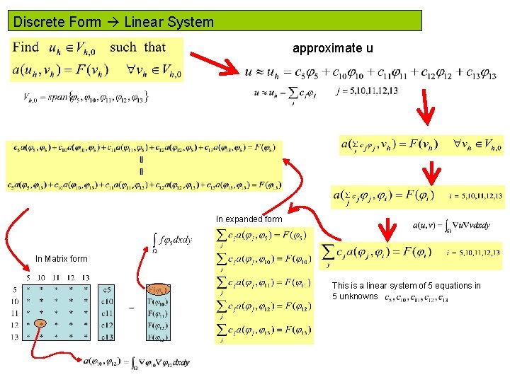
Discrete Form Linear System approximate u In expanded form In Matrix form This is a linear system of 5 equations in 5 unknowns

The approximate Solution In Matrix form Once this linear system is solved we obtain an approximation to the solution Remark: We are going to focus our attention in the efficient construction of this stiffness matrix

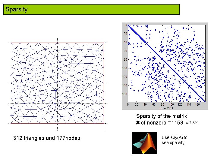
Sparsity In Matrix form Remark: This matrix is sparse (many zeros) few non-zero entries another example

Sparsity of the matrix # of nonzero =1153 312 triangles and 177 nodes Use spy(A) to see sparsity

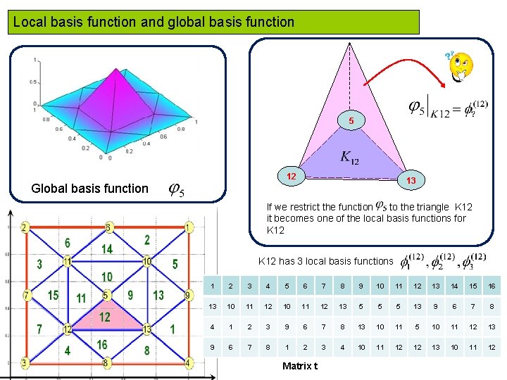
Local basis function and global basis function 5 12 Global basis function 13 If we restrict the function to the triangle K 12 it becomes one of the local basis functions for K 12 has 3 local basis functions 1 2 3 4 5 6 7 8 9 10 11 12 13 14 15 16 13 10 11 12 13 5 5 5 13 9 6 7 8 4 1 2 3 9 6 7 8 13 10 11 5 10 11 12 13 9 6 7 8 1 2 3 4 10 11 12 12 13 10 11 12 Matrix t

Remark: This matrix is sparse (many Assembly of the Stiffness Matrix zeros) few non-zero entries Remark: In Matrix form Remark: nonzero entry is a sum of integrals of local basis functions over a triangle These few nonzero entries are computed by looping over all triangles 1 2 3 4 5 6 7 8 9 10 11 12 13 14 15 16 13 10 11 12 13 5 5 5 13 9 6 7 8 4 1 2 3 9 6 7 8 13 10 11 5 10 11 12 13 9 6 7 8 1 2 3 4 10 11 12 12 13 10 11 12

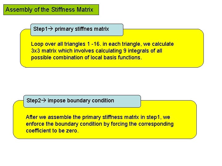
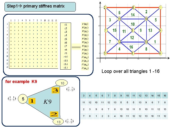
Assembly of the Stiffness Matrix Step 1 primary stiffnes matrix Loop over all triangles 1 -16. in each triangle, we calculate 3 x 3 matrix which involves calculating 9 integrals of all possible combination of local basis functions. Step 2 impose boundary condition After we assemble the primary stiffness matrix in step 1, we enforce the boundary condition by forcing the corresponding coefficient to be zero.

Step 1 primary stiffnes matrix For k = 1 : 16 Step 1 a: Step 1 b: Step 1 c: End the loop find all gradients Find 9 integrals Add these contributions to the primary stiffness matrix

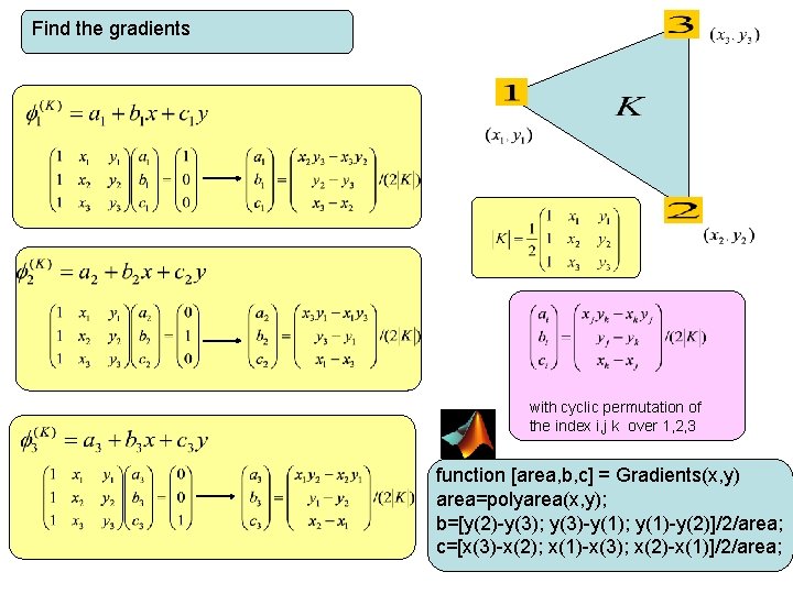
Find the gradients with cyclic permutation of the index i, j k over 1, 2, 3

Find the gradients with cyclic permutation of the index i, j k over 1, 2, 3 function [area, b, c] = Gradients(x, y) area=polyarea(x, y); b=[y(2)-y(3); y(3)-y(1); y(1)-y(2)]/2/area; c=[x(3)-x(2); x(1)-x(3); x(2)-x(1)]/2/area;

Step 1 primary stiffnes matrix Loop over all triangles 1 -16 for example K 9 10 5 13 1 2 3 4 5 6 7 8 9 10 11 12 13 14 15 16 13 10 11 12 13 5 5 5 13 9 6 7 8 4 1 2 3 9 6 7 8 13 10 11 5 10 11 12 13 9 6 7 8 1 2 3 4 10 11 12 12 13 10 11 12

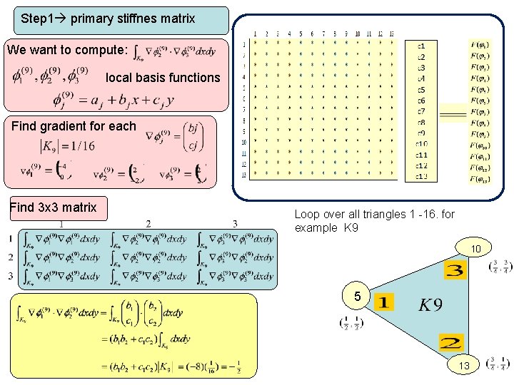
Step 1 primary stiffnes matrix We want to compute: local basis functions Find gradient for each Find 3 x 3 matrix Loop over all triangles 1 -16. for example K 9 10 5 13

Step 1 primary stiffnes matrix We want to compute: local basis functions Find gradient for each Find 3 x 3 matrix 10 l oba l g o 5 al t Loc 13

Step 1 primary stiffnes matrix Triangle K 10 al to glo b al 2 3 -1/2 1/2 0 0 1/2 5 10 11 5 1 -1/2 10 -1/2 0 11 -1/2 0 1/2 Lo c 1 2 3 1 1 -1/2

K =1 1/2 0 -1/2 K =13 0 1/2 -1/2 1 K =2 1/2 0 -1/2 0 1/2 -1/2 1 -1/2 1 1/2 0 -1/2 0 1/2 -1/2 -1/2 1 0 1/2 -1/2 1 K =15 0 1/2 -1/2 1 K =4 1/2 0 -1/2 0 1/2 -1/2 K =14 K=3 1/2 0 -1/2 K =16 0 1/2 -1/2 1 1/2 0 -1/2

Step 1 primary stiffnes matrix 1 0 0 0 0 0 0 4 0 0 0 2 0 0 0 0 0 -1 0 0 0 -1 -1 0 0 -1 -1 0 0 0 0 2 0 0 0 0 -1 -1 0 0 0 0 -1 -1 -1 0 0 0 -1 2 -1 0 0 -1 4 0 0 0 0 4 -1 0 0 0 -1 -1 0 0 0 4 function A = Stiff. Mat 2 D(p, t) np = size(p, 2); nt = size(t, 2); A = sparse(np, np); for K = 1: nt loc 2 glb = t(1: 3, K); % local-to-global map x = p(1, loc 2 glb); % node x-coordinates y = p(2, loc 2 glb); % node y[area, b, c] = Gradients(x, y); AK = (b*b'+c*c')*area; % element stiff mat A(loc 2 glb, loc 2 glb) = A(loc 2 glb, loc 2 glb)+ AK; % add element stiffnesses to A end 1 2 3 4 5 6 7 8 9 10 11 12 13 14 15 16 13 10 11 12 13 5 5 5 13 9 6 7 8 4 1 2 3 9 6 7 8 13 10 11 5 10 11 12 13 9 6 7 8 1 2 3 4 10 11 12 12 13 10 11 12

Assemble the Load vector L In Matrix form 1 2 3 4 5 6 7 8 9 10 11 12 13 14 15 16 13 10 11 12 13 5 5 5 13 9 6 7 8 4 1 2 3 9 6 7 8 13 10 11 5 10 11 12 13 9 6 7 8 1 2 3 4 10 11 12 12 13 10 11 12

Assembly of the Load Vector Step 1 primary Load vector Loop over all triangles 1 -16. in each triangle, we calculate 3 x 1 matrix which involves calculating 3 integrals Step 2 impose boundary condition After we assemble the primary load vector and stiffness matrix in step 1, we enforce the boundary condition by forcing the corresponding coefficient to be zero.

Step 1 primary Load vector Loop over all triangles 1 -16. in each triangle, we calculate 3 x 1 matrix which involves calculating 3 integrals The load vector b is assembled using the same technique as the primary stiffness matrix A, that is, by summing element load vectors BK over the mesh. On each element K we get a local 3× 1 element load vector BK with entries BKi = ∫Kf φi dx; i = 1; 2; 3 Using node quadrature, we compute these integrals we end up with BKi≈ 1/3 f (Ni)|K|; i = 1; 2; 3 2

Step 1 primary Load vector Loop over all triangles 1 -16. in each triangle, we calculate 3 x 1 matrix which involves calculating 3 integrals 1 2 3 4 5 6 7 8 9 10 11 12 13 14 15 16 13 10 11 12 13 5 5 5 13 9 6 7 8 4 1 2 3 9 6 7 8 13 10 11 5 10 11 12 13 9 6 7 8 1 2 3 4 10 11 12 12 13 10 11 12

Step 1 primary Load vector Loop over all triangles 1 -16. in each triangle, we calculate 3 x 1 matrix which involves calculating 3 integrals We summarize the computation of the load vector with the following Matlab code. b 1 = 0 0 1/256. . . b 16 = 1/256 3/256 1/96 0 0 1/24 0 1/48 0 1/32 0 1/128 3/128 9/128 3/128 function b = Load. Vec 2 D(p, t) f = inline('x. *y'); np = size(p, 2); nt = size(t, 2); b = zeros(np, 1); for K = 1: nt loc 2 glb = t(1: 3, K); x = p(1, loc 2 glb); y = p(2, loc 2 glb); area = polyarea(x, y); b. K = [f(x(1), y(1)); f(x(2), y(2)); f(x(3), y(3))]/3*area % element load vector b(loc 2 glb) = b(loc 2 glb)+ b. K; % add element loads to b end

Step 2 impose boundary condition 1 0 0 0 0 0 0 4 0 0 0 2 0 0 0 0 0 -1 0 0 0 -1 -1 0 0 -1 -1 0 0 0 0 2 0 0 0 0 -1 -1 0 0 0 0 -1 -1 -1 0 0 0 -1 2 -1 0 0 -1 4 0 0 0 0 4 -1 0 0 0 -1 -1 0 0 0 4 c 1 c 2 c 3 c 4 c 5 c 6 c 7 c 8 c 9 c 10 c 11 c 12 c 13 = 0 0 1/24 0 1/48 0 1/32 0 1/128 3/128 9/128 3/128 We want to impose the boundary conditions

Step 2 impose boundary condition Rearrange the columns and the code by starting with the interior nodes then list the boundary nodes 5 10 11 12 13 1 2 3 4 6 7 8 9 4 -1 -1 0 0 0 0 -1 4 0 0 0 -1 -1 0 4 0 0 0 -1 -1 0 0 4 0 0 0 -1 -1 0 0 0 1 0 0 0 0 0 -1 0 0 0 0 0 -1 0 0 0 0 0 -1 -1 0 0 0 2 0 0 0 0 0 -1 -1 0 0 0 2 0 0 -1 0 0 0 0 2 c 5 c 10 c 11 c 12 c 13 c 1 c 2 c 3 c 4 c 6 c 7 c 8 c 9 = 1/48 1/128 3/128 9/128 3/128 0 0 1/24 0 0 1/32 0

Step 2 impose boundary condition This can be done in Matlab: function [A, b] = impose_boundary(A, b, p, t, e, bound, inter); np = size(p, 2); % total number of nodes b = b(inter); % modify load vector A = A(inter, inter); % modify stiffness matrix Main. m files load sample_mesh np = size(p, 2); bound = unique([e(1, : ) e(2, : )]); inter = setdiff([1: np], bound); % boundary nodes % interior nodes A = Stiff. Mat 2 D(p, t); b = Load. Vec 2 D(p, t); [A, b] = impose_boundary(A, b, p, t, e, bound, inter); c = zeros(np, 1); % allocate solution vector c(bound) = sparse(length(bound), 1); % boundary nodes solution c(inter) = Ab; % solve the linear system x=0: 0. 01: 1; y=0: 0. 01: 1; u=tri 2 grid(p, t, c, x, y); mesh(x, y, u) % plot surface 0 0 5/288 0 0 29/4608 47/4608 101/4608 47/4608

Step 2 impose boundary condition This can be done in Matlab: u =tri 2 grid(p, t, c, 1/2, 1/8) 0 0 5/288 0 0 29/4608 47/4608 101/4608 47/4608

Step 2 impose boundary condition x=0: 0. 01: 1; y=0: 0. 01: 1; u=tri 2 grid(p, t, c, x, y); mesh(x, y, u)

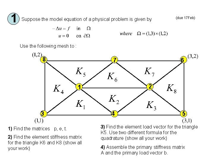
1 Suppose the model equation of a physical problem is given by (due 17 Feb) Use the following mesh to : 8 7 2 1 3 1) Find the matrices p, e, t. 2) Find the element stiffness matrix for the triangle K 6 and K 8 (show all your work) 6 4 5 3) Find the element load vector for the triangle K 5. Use two different formula for the quadrature (show all your work) 4) Assemble the primary stiffness matrix A and the primary load vector b.