Discrete Event Simulation Represents the stochastic nature of

Discrete Event Simulation • Represents the stochastic nature of the system being modeled • Driven by the occurrence of events

Discrete Event Simulation • Primary event – an event which occurrence is scheduled at a certain time • Conditional event an event triggered by a certain condition becoming true

Discrete Event Simulation • The future event list (FEL) … – Controls the simulation – Contains all future events that are scheduled – Is ordered by increasing time of event notice – Contains only primary events • Example FEL for some simulation time t≤T 1: (t 1, Event 1) (t 2, Event 2) t 1≤ t 2≤ t 3≤ t 4 (t 3, Event 3) (t 4, Event 4)

Discrete Event Simulation • Operations on the FEL: – Insert an event into FEL (at appropriate position) – Remove first event from FEL for processing – Delete an event from the FEL • The FEL is thus usually stored as a linked list • The simulator spends a lot of time processing the FEL – Efficiency is thus very important!

DES yes FEL empty? no Remove and process first primary event Process conditional event yes Conditional event enabled? no

DES • Simulation clock register virtual time, not real time • Can simulate one century in a second

DES Simulation clock: (t 4, Arrival) t 2 (t 3, Service complete)

How To Generate A Random Variable? • Linear congruential method • Xn+1 = (a Xn + c) modulo m

Random Variable Generation • Let X 0 = a = c = 7, and m = 10 • This gives the pseudo-random sequence {7, 6, 9, 0, …} • What went wrong? • The choice of the values is critical to the performance of the algorithm • Also demonstrates that these methods always “get into a loop”

Multiplicative Congruential Method • • • -c=0 period reduced, faster Xn = (X 0+nc) modulo m a = 16807 m = 2147483647 e=0 X 0 = 314159

Random Variate Generation • We have a sequence of pseudo-random uniform variates. How do we generate variates from different distributions? • Random behavior can be programmed so that the random variables appear to have been drawn from a particular probability distribution • If f(x) is the desired pdf, then consider the CDF • This is non-decreasing and lies between 0 and 1

Random Variate Generation • Given a sequence of random numbers ri distributed over the same range (0, 1) • Let each value of ri be a value of the function Fx(x) • Then the corresponding value xi is uniquely determined • The sequence xi is randomly distributed and has the probability density function f(x)

Random Variate Generation

Random Variate Generation

Method of Inverse • For the exponential distribution • For positive xi • Thus

Method of Inverse • Note that ri has the same distribution as 1 -ri so we would in reality use • Other random variates can be derivated in a similar fashion.

Other Methods • Composition – sum of independent random variables (example: Erlang) • Rejection-acceptance – generate and test

Simulation: A Statistical Experiment

Steady State Distribution

Simulating a Queue Simulation clock: Arrival Service interval complete 5 5 1 6 3 9 3 12 15 Customer Begin Service arrives service 5 7 11 14 15 2 4 3 1 duration

Computing Statistics Average waiting time for a customer: (0+1+2+2)/4=1. 25 Arrival Service interval duration 5 5 1 6 3 9 3 12 Customer Begin Service arrives complete ¬ 0® ¬ 1® ¬ 2® service 5 7 11 14 2 4 3 1 7 11 14 15

Computing Statistics P(customer has to wait): =3/4=0. 75 Arrival Service interval duration 5 5 1 6 3 9 3 12 Customer Begin Service arrives complete 5 ¬W® ¬W® service 2 7 11 14 7 4 3 1 11 14 15

Computing Statistics P(Server busy): 10/15=0. 66 Arrival Service interval duration 5 5 1 6 3 9 3 12 Customer Begin Service arrives complete 5 7 11 14 service 2 4 3 1 7 11 14 15

Computing Statistics Average queue length: =(1*1+2*1)/15=0. 33 Arrival Service interval duration 5 5 1 0® 6 11 3 0® 9 14 Customer Service arrives complete 0® 5 1® 7 Begin 2 4 1® 11 3 service 7

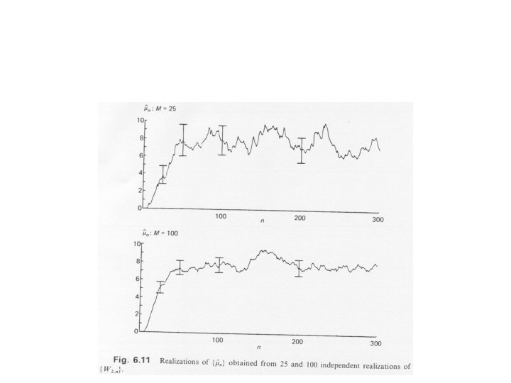
Independent Replications • Generate several sample paths for the model which are statistically independent and identically distributed. • Reset the model performance measures at the beginning of each replication, • And use a different random number seed for each independent replication

Independent Replications • Distributions of the performance measures can then be assumed to have finite mean and variance • With sufficient replications the average over the replications can be assumed to have a Normal distribution

Statistical Analysis of Results • Given that each independent replication of a simulation experiment will yield a different outcome… • To make a statement the about accuracy we have to estimate the distribution of the estimator • Need to determine that the distribution becomes asymptotically centered around the true value

Statistical Analysis of Results • Cannot be established with certainty in the case of a finite simulation • The usual method used to estimate variability is to produce “confidence interval” estimates

Confidence Intervals • Given some point estimate p a we produce a confidence interval (p-d, p+d) • The “true” value is estimated to be contained within the interval with some chosen probability, e. g. 0. 9 • The value d depends on the confidence level – the greater the confidence, the larger the value of d

Confidence Intervals • Let x 1, x 2, …, xn be the values of a random sample from a population determined by the random variable X • Let the mean of X be m=E(X) and variance s 2 • Assume: either X is normally distributed or n is large • Then: by the law of large numbers, X» normally distributed

Confidence Intervals • Then, given s the 100(1 -a)% confidence interval is given by • Where (2) • za is defined to be the largest value of z such that P(Z>z)=a and Z is the standard normal random variable

Confidence Intervals • Can be taken from tables of the normal distribution • For example, for a 95% confidence interval a=0. 05 and za/2=z 0. 025=1. 96

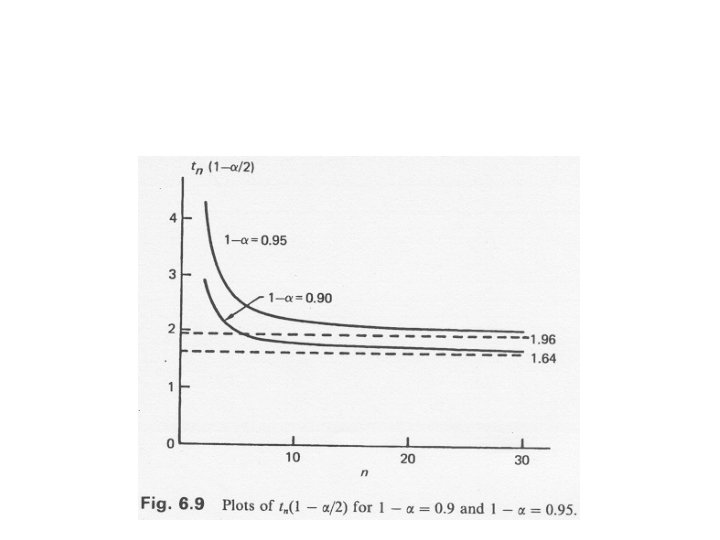
Using Student`s T • When we know neither m nor s we can use the observed sample mean x and sample standard deviation s • If n is large then we simply use s for s in Equation (2). • If n is small and X is normally distributed then we may use

Using Student`s T • ta/2 is defined by P(T>ta/2)=a/2 • T has a Student-t distribution with n-1 degrees of freedom • This is the more frequently used formula in simulation models

Confidence Interval

Batch Means