Discrete Event Simulation 1 Discrete Event Simulation Imitating

Discrete Event Simulation 1

Discrete Event Simulation • Imitating the operation of a system over time. • Typical objective- Support decisions related to the use of limited resources. 2

Discrete Event Simulation - Outline • To understand how and why we simulate such systems we will cover: – Analysis options. – The mechanics of how a simulation is implemented on a computer. • Terminology • Manual execution of a discrete event simulation • Performance measures – The steps of a simulation study. – Analyzing input and output data. – Simulating randomness. 3

Analysis Options • Utilize the simplest fastest methods that provide adequate decision support. • What are the analysis objectives? – What/How many parameters and variables are being explored – What is the system complexity? – How much precision is required? 4

Analysis Options • Resource allocation decisions – It may suffice to examine resource utilizations and WIP. Note that utilization is a percent, or ratio 5

15 JPH each Example Jobs arriving 25 JPH Total workstation JPH = 15 + 15 • A workstation has two machines in parallel that can process jobs at a rate of 15 JPH. Jobs arrive over time at a rate of 25 JPH.

Analysis Options • Unless a system has very high relative variability, utilizations < 90% will lead to “reasonable” queue sizes. – Demo Exponential arrivals/processing medium/high variability What is very high variability? • Broken tools and long downtimes • Specialty jobs or processing times • Worker expertise causing errors These are common occurrences in a real factory. Some amount of downtown needs to be planned for. 7

In-class Exercise • Two types of jobs (A and B) arrive to a single machine for processing. The arrival rate of type A jobs is 5 per hour, and 2. 5 per hour for type B jobs. Type A jobs have an average service time of 5 minutes, and type B jobs have an average service time of 11 minutes. – What is the utilization of the machine?

7/7 announcements • Will answer any review questions next class • Midterm Exam 1 Thursday 9 am (no lecture) – Taken remotely, questions delivered through Canvas • Lab and weekly reflection due Thursday 10 pm • Lab Exam 1 next week Monday 9 am (no lecture) – Taken remotely, questions delivered through Canvas

Analysis Options • At the next level of detail queuing models may be applied. – More information than utilization calculations. – Difficult skill to apply. – Some G/G/m models were covered in IE 368. • Get more information than just utilization or average number in queue • More than 1 processing step in a row? • Complex custom job shop flow? 11

Discrete Event Simulation - Basics • Fundamental components/terminology. • Simulation mechanics – Manual execution of a simulation. • Performance measures. 12

Terminology • We will simulate stochastic dynamic discrete-event systems. – Stochastic – Randomness over time • Deliveries, job arrivals • Operation times • Machine failures – Dynamic – The passage of time is part of the simulation • Productions lines • Service centers 13

Terminology • Discrete event – the system state (finite) only changes when events occur. Events only occur at specific time points – System state – A set of numerical values with the necessary information to describe a system for analysis purposes. – Examples Job shop with m machines ni = # of jobs at machine i for i = 1, 2, …, m si = status of machine i (0 = down, 1 = up) for i = 1, 2, …, m System state = [(n 1, s 1), (n 2, s 2), …, (nm, sm)] 14

Terminology • Entities – Objects that move through the simulated system. – Examples Parts, customers, orders, jobs, lots, … • Entities can be combined and split. 15

Terminology • Attributes – Parameters, data specific to an entity. – Examples Arrival times, part types, processing times, … – The same concept as objects (entities) and object data (attributes) in Object Oriented Programming 16

Terminology • Global variables/parameters – System wide values accessible by all entities and resources. – Examples Simulation time Queue sizes – Resources – Items that are used by entities and found in limited amounts. – Queues – Spaces where entities wait for resources. 17

Terminology • Events – Actions that cause the system state to change. – Examples Job shop example: Job arrivals Job completions Machine failures Machine repairs 18

Mechanics of Simulation • Event calendar and the passage of simulated time. – Simulations maintain an event calendar that functions like the control center of the simulation. – The event calendar is a time sorted list of events and the times that they occur. – When the event at the top of the list occurs, simulated time is advanced and specific logic is initiated. • This logic changes the state, updates statistics, and schedules additional events. 19

Event Calendar Main Procedures/ Functions Execute the appropriate functions/procedures for that event type (job arrival, job completion, …) Computer Program 20

Simulation Clock • Simulation time does not advance uniformly unless controlled. x x x 21

Manual Simulation • We will execute a manual simulation on paper to understand the fundamentals of simulation mechanics. • You will execute what the computer carries out in a simulation. 22

Example System • A “single server queuing system with infinite queue capacity”. • System description – Customers (jobs) arrive one at a time to be processed by a server who can serve a single customer at a time. If the server is idle when a customer arrives the customer immediately starts service, otherwise the customer waits in an infinite capacity queue and is served in first-in-firstout (FIFO) order. 23

Example System … Arrivals Queue Server For some fixed simulated time: • How many customers are processed? • What’s the average customer queue time? • What’s the average customer system time? • What is the average number in queue? • What is the server utilization? • What are max observed values for • Queue time? • Time in system? • Number in queue?

Manual Simulation • Will use pseudo code and a table to implement the simulation. • See handout. 25

7/8 announcements • • HW 2 graded Lab and weekly reflection due Thursday 10 pm Participation questions due Thursday 10 pm Midterm exam 1 Thursday during class 9 am – No lecture • Lab exam 1 Monday during class 9 am – No lecture • Review now

Notation t = simulation time tbefore = prior event simulation time. Q(t) = # in queue at time t B(t) = 1 if the server is busy, and 0 if the server is idle P = the number of customers/jobs processed after each event N = the number of customers/jobs that have passed through the queue ∑WQ = the sum of the queue times observed for customers WQ* = Max queue time observed ∑TS = the sum of the system times (queue + service) observed for customers TS* = Max system time observed ∫Q = the area under the Q(t) curve through time t Q* = Max value for the number in queue observed ∫B = the area under the B(t) curve through time t

Pseudocode • See Canvas

7/14 announcements • Lab 3 results very good. Feedback shows big strides in feeling more confident with Monte Carlo simulation. Good work class! • Midterm Exam results posted. – Contact me to set up an appointment to review your results • Lab 4 and weekly reflection due Thursday 10 pm • HW 3 due Monday 10 pm

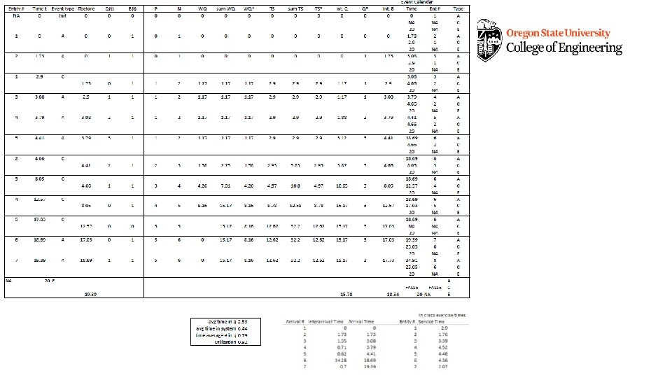
Manual Simulation Table

pr nd ax M er Q (t) th # in ro Q ug h Ar tim ea u e t nd er B (t) th ro ug h tim e t u ea Ar oc es se # d pa ss ed th To ro ug ta l o h Q f a ll t im M es ax in Q Q ti m e To ta l o f a ll t M im ax es ti in m e sy in st sy em st em # m es ti al riv ar ity En t 0 1 if id if le bu sy Q in #

pr nd ax M er Q (t) th # in ro Q ug h Ar tim ea u e t nd er B (t) th ro ug h tim e t u ea Ar oc es se # d pa ss ed th To ro ug ta l o h Q f a ll t im M es ax in Q Q ti m e To ta l o f a ll t M im ax es ti in m e sy in st sy em st em # m es ti al riv ar ity En t 0 1 if id if le bu sy Q in #

7/15 announcements • Lab 4 and weekly reflection due Thursday 10 pm • Weekly Canvas Participation questions due Thursday 10 pm • HW 3 due Monday 10 pm • Next week I am attending a remote conference on Thursday during our regular lab time (July 23) – I will set up a poll for people to respond for alternate options

pr nd ax M er Q (t) th # in ro Q ug h Ar tim ea u e t nd er B (t) th ro ug h tim e t u ea Ar oc es se # d pa ss ed th To ro ug ta l o h Q f a ll t im M es ax in Q Q ti m e To ta l o f a ll t M im ax es ti in m e sy in st sy em st em # m es ti al riv ar ity En t 0 1 if id if le bu sy Q in #

Q(t) 0 Simulation time B(t) 1 0

“Simulation Performance Measures” • Simulation performance measures – Several different types – Tally statistics –”Tally” is an Arena term. • Sample average • Data is collected on a performance measure with individual outcomes 37

“Simulation Performance Measures” • Simulation performance measures. – Counters – Incremented when specific events occur. • E. g. , Completed jobs. – Time average measures – Arena calls these “Time persistent” • Variables are weighted by the length of time that they occur 38

“Simulation Performance Measures” • Simulation performance measures. – Maximums and minimums – Changed when specific comparisons indicate. • E. g. , Maximum jobs in queue. 39

“Simulation Performance Measures” • The average time a part spends in the system. – Tally or Time average (persistent)? • Utilization of a machine. – Tally or Time average (persistent)? 40

In-class Exercise No entities have 0 time in queue • Compute the average number in queue, and average time in queue through T = 14 (assume first-in-first-out).

In-class Exercise

Simulation Modeling Views • The manual simulation looked at the system dynamics by examining the events that occur. – This is called event orientation. • Event orientation – Define the system state – Identify all events that change the state • Program the logic associated with each event 43

Simulation Modeling Views • Process orientation – The focus on defining the system dynamics is on entities and how they flow through the system. • Manual simulation. – Arrive-> Queue -> Machine -> Depart • Arena is process orientated simulation system. • Process orientation tends to be easier when modeling large systems. • Most simulations are implemented in an event driven manner (including Arena). 44

7/16/2020 announcements • Lab 4 and weekly reflection due today 10 pm • Weekly Canvas Participation questions due today 10 pm • HW 3 due Monday 10 pm • Next week I am attending a remote conference on Thursday during our regular lab time (July 23) – Poll set up in Canvas – respond by Monday 10 pm

Initial Steps in a Simulation Study • Define the objectives of the study. – Why is the simulation needed • Define performance measures needed • Write a description of the system. – Verbal description, flow chart • List assumptions if any. • Write a report introduction. • From the system description identify – Data collection needs • Random Variables • Parameters 46

Intermediate Steps • Begin model development. • Fit distributions to data for use in the model. • Verify and validate the model. • Experimentation and analysis. 47

Final Steps • Report writing. • Presentations. – Animation if necessary • Other points. – On going communication throughout the study. – Observation/face time. 48