Discrete Convolution of Two Signals In this animation

Discrete Convolution of Two Signals In this animation, the discrete time convolution of two signals is discussed. Convolution is the operation to obtain response of a linear system to input x[n]. Considering the input x[n] as the sum of shifted and scaled impulses, the output will be the superposition of the scaled responses of the system to each of the shifted impulses. Course Name: Signals and Systems Level: UG Authors Phani Swathi Mentor Prof. Saravanan Vijayakumaran

Learning Objectives After interacting with this Learning Object, the learner will be able to: • Explain the convolution of two discrete time signals

1 2 Definitions of the components/Keywords: Convolution of two signals: The x[n] and h[n] are the two discrete signals to be convolved. The convolution of two signals is denoted by which means 3 4 5 where k is a dummy variable.

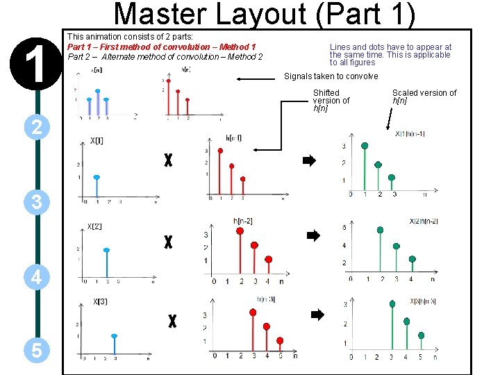
Master Layout (Part 1) 1 2 3 4 5 This animation consists of 2 parts: Part 1 – First method of convolution – Method 1 Part 2 – Alternate method of convolution – Method 2 Lines and dots have to appear at the same time. This is applicable to all figures Signals taken to convolve Shifted version of h[n] Scaled version of h[n]

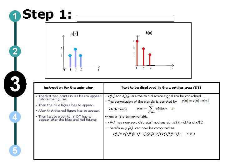
1 Step 1: 2 3 Instruction for the animator • The first two points in DT has to appear before the figures. • Then the blue figure has to appear. 4 • After that the red figure has to appear. • Then last two points in DT has to appear after the blue and red figures. Text to be displayed in the working area (DT) • x[n] and h[n] are the two discrete signals to be convolved. • The convolution of the signals is denoted by which means where k is a dummy variable. • x[n] has non-zero discrete impulses at x[1], x[2] and x[3]. • Therefore, y [n] can now be computed as y[n]= x[1]h[n-1]+x[2]h[n-2]+x[3]h[n-3] ; 5 n≥ 1

1 Step 2: Overall calculation of y[n] X[1]h[n-1] 3 2 2 1 0 h[n-2] 3 2 3 n X[2]h[n-2] 6 3 2 4 1 2 0 1 2 3 4 n h[n-3] 0 1 2 3 4 3 n X[3]h[n-3] 3 4 2 2 1 1 0 Instruction for the animator 5 1 1 2 3 4 5 n 2 5 n Text to be displayed in the working area (DT) • The figures has to appear row wise. First the blue fig. then red fig. and then the green figure has to appear. • x[n] has non-zero discrete impulses at x[1], x[2] and x[3]. • After the 9 figures appear row wise, all the fig. should appear at a time in the fashion shown above. • From definition, y[n] is the superposition of the scaled responses of the system to each of the shifted impulses. • The summation of all the products of x[k]h[n-k] gives y[n].

1 Step 3: X[1]h[n-1] x[1]h[n-1] 3 2 1 0 Instruction for the animator • Show the fig in red and then X[1]h[n-1] has to appear 4 5 1 2 3 n Text to be displayed in the working area (DT) • The response due to the input x[k] applied at time k • The time shift of h[n] is taken • Then the green figure has to appear • Then scaling of h[n-1] with x[1] is done. • After that the sentence “the scaled signal x[1]h[n-1]” should appear • The signal x[1]h[n-1] is the same as h[n-1] since x[1]=1.

1 Step 4: X[2]h[n-2] X[2] h[n-2] 6 5 4 2 3 3 3 2 2 1 1 0 1 2 3 4 n Instruction for the animator • First show the figure in red and then labeling h[n-2] should appear • Then the green figure has to appear 4 5 • After that the sentence “the scaled signal x[2]h[n-2]” should appear 0 1 2 3 4 n Text to be displayed in the working area (DT) • The next time shift of h[n-1] is taken • Then scaling of h[n-2] with x[2] is done. • The signal x[2]h[n-2] is the doubled version of h[n-2] since x[2]=2.

1 Step 5: X[3]h[n-3] 2 3 3 3 2 2 1 1 0 1 2 3 4 5 Instruction for the animator • First show the figure in red and then 4 5 x[3]h[n-3] labeling h[n-3] should appear • Then the green figure has to appear • After that the sentence “the scaled signal x[3]h[n-3]” should appear n 0 1 2 3 4 5 n Text to be displayed in the working area (DT) • The next time shift of h[n-3] is taken • Then scaling of h[n-3] with x[3] is done. • The signal x[3]h[n-3] is the same as h[n-3] since x[3]=1.

1 Step 6: Y[n] 8 7 6 2 5 4 3 3 4 5 2 1 0 1 2 3 4 5 6 7 8 n Instruction for the animator Text to be displayed in the working area (DT) • First the symbol y[n] must appear and then the figure in green must appear. • The output of the system y[n] =x[1]h[n-1]+x[2]h[n-2]+x[3]h[n-3]

Electrical Engineering Use STAM template Slide 1 Introduction Slide 3 Definitions Slide 26 Slide 28 Slide 27 Want to know more… Test your understanding Lets Sum up (summary) (Further Reading) (questionnaire) Analogy Interactivity: The correct answer is shown in red Try it yourself Fig. A Fig. B Fig. C Fig. 1 Fig. 2 Demo Activity Fig. A Fig. B Fig. C 11 Instructions/ Working area Credits

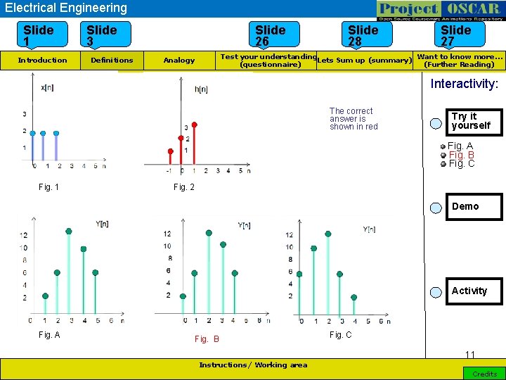
Interactivity option 1: 1 Step No 1: y[n] x[n] h[n] 3 2 2 3 1 3 4 5 0 3 2 1 2 3 4 5 0 1 Fig. 1 0 2 3 4 5 1 Fig. 2 1 2 Fig. 1 3 Interactivit y type (IO 1/IO 2) Instruction to learners Choose from fig. A, B & C. Find the convolution of x[n] and h[n] 4 5 n -1 0 1 2 3 Fig. 2 Boundary limits & options Instruction to animators Results and output • Show fig 1, fig. 2 in the question part. • show fig. B as the output. 4 5 n

Interactivity option 1: 1 Step No 2: y[n] 2 Y[n] 12 12 103 10 82 8 6 6 4 4 1 3 20 1 5 3 4 5 0 1 Fig. 1 0 Interactivit y type (IO 1/IO 2) 4 2 1 2 3 4 5 2 Fig. 2 2 3 4 a) Fig. A Instruction to learners Find the convolution of x[n] and h[n] 5 6 n 0 1 2 3 4 b) Fig. B Boundary limits & options Instruction to animators Results and output • Show fig. A, fig. B and fig. C as the options • show fig. B as the output. 5 6 n

Interactivity option 1: 1 Step No 3: y[n] Y[n] 12 3 2 10 8 2 6 1 3 0 4 12 2 5 4 5 0 1 Fig. 1 2 3 4 5 Fig. 2 0 1 2 c) Fig. C Interactivit y type (IO 1/IO 2) 4 3 Instruction to learners 3 4 Boundary limits & options 5 6 n Instruction to animators Results and output • show option B as the output. • If the user chooses ‘B’ remark “correct answer” should appear if not “wrong answer” should appear.

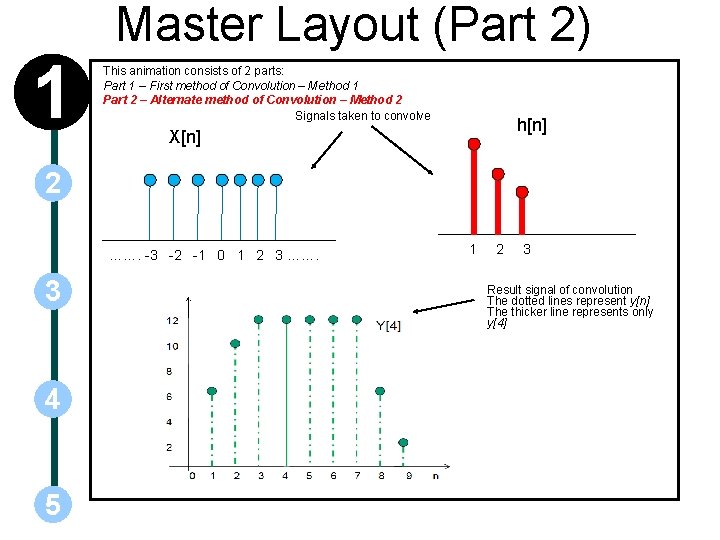
Master Layout (Part 2) 1 This animation consists of 2 parts: Part 1 – First method of Convolution – Method 1 Part 2 – Alternate method of Convolution – Method 2 Signals taken to convolve h[n] X[n] 2 ……. -3 -2 -1 0 1 2 3 ……. 3 4 5 1 2 3 Result signal of convolution The dotted lines represent y[n] The thicker line represents only y[4]

1 Step 1: X[n] h[n] 2 2 3 …. -3 -2 -1 0 1 2 3…. . Instruction for the animator • First sentence in DT is to appear before the figures. • Then the blue fig. has to appear and then the red fig. 4 5 • The text in last two sentences in DT has to appear after the blue figure. 1 2 3 n Text to be displayed in the working area (DT) • x[n] and h[n] are the two signals taken to convolve. • x[k] has 7 non-zero impulses from -3 to +3 with an amplitude of 2. so, it is difficult to use method 1. • Then Y[n] is calculated using formula.

1 Step 2: h[n-k] X[k] 3 2 1 2 3 4 5 -3 -2 -1 2 k=n-1 k= n 0 1 2 3 Instruction for the animator k Text to be displayed in the working area (DT) • First the blue fig. has to appear then the red fig. • h[n-k] is the time reversal and shifted version of h[n] as shown in the figure. • The text in first two sentences in DT has to appear after the blue figure. • h[n-k] is • The sentences from 3 onwards in DT should appear after the red fig. • h[n-k] h[0] when k= n • Similarly, h[n-k] is h[1] when k=n-1 is h[2] when k= n-2 and so on.

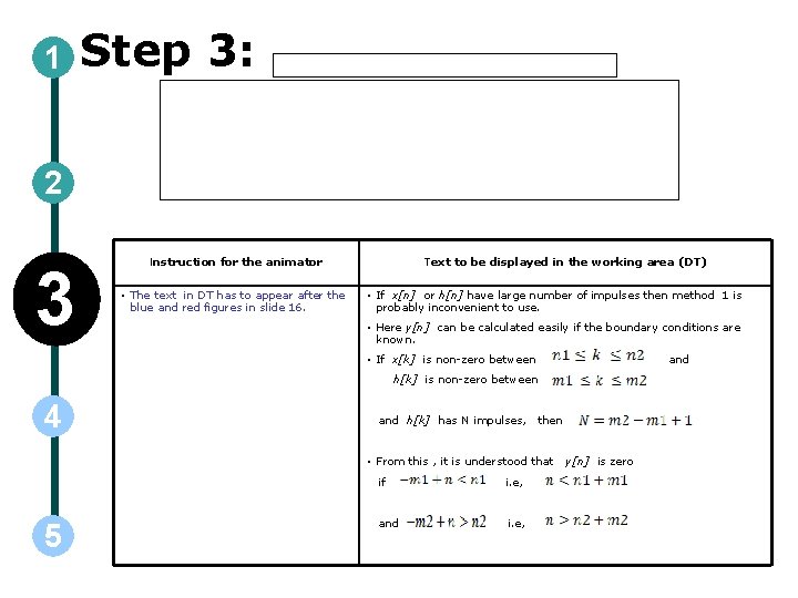
1 Step 3: 2 3 Instruction for the animator • The text in DT has to appear after the blue and red figures in slide 16. Text to be displayed in the working area (DT) • If x[n] or h[n] have large number of impulses then method 1 is probably inconvenient to use. • Here y[n] can be calculated easily if the boundary conditions are known. • If x[k] is non-zero between and h[k] is non-zero between 4 and h[k] has N impulses, then • From this , it is understood that 5 if i. e, and i. e, y[n] is zero

1 Step 4: X[k] h[4 -k] 2 3 -3 -2 -1 0 1 2 3 Instruction for the animator • First the blue fig. and then the red fig. has to appear. • The text in DT has to appear after the red fig. 4 5 2 3 4 k Text to be displayed in the working area (DT) • h[4 -k] is the time reversal and shifted version of h[n] as shown in the figure.

1 Step 5: X[k]h[4 -k] 6 4 2 2 3 2 Instruction for the animator • The text in DT has to appear after the red fig. 5 4 Text to be displayed in the working area (DT) • Y[4] can be calculated by summing all the values of product of x[k]h[4 -k]. i. e, 4 3

1 Step 6: Y[4] 12 Y[4] 10 2 8 6 4 3 4 2 0 1 2 Instruction for the animator 4 5 6 7 8 9 n Text to be displayed in the working area (DT) • First the symbol y[4] must appear and then the figure in green must appear. • For example, to find y[4] • Both the lines and the balls should appear at a time. • That is given as • After the figure, the text in DT has to appear. 5 3 • The output of the system y[4] is the summation of x[k]h[n-k] y[4] = x[0]h[4 -0]+x[1]h[4 -1]+x[2]h[4 -2]+x[3]h[4 -3]+x[4]h[4 -4] • The dotted lines represent the solution for y[n].

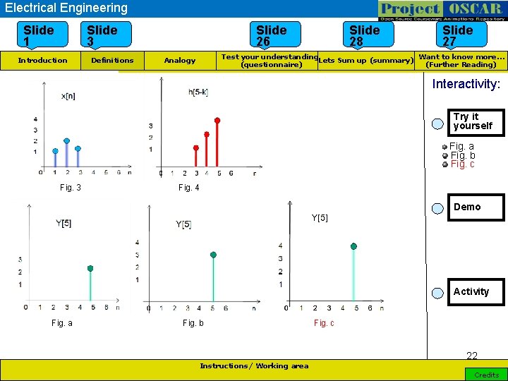
Electrical Engineering Use STAM template Slide 1 Slide 3 Introduction Definitions Slide 26 Slide 28 Slide 27 Want to know more… Test your understanding Lets Sum up (summary) (Further Reading) (questionnaire) Analogy Interactivity: Try it yourself Fig. a Fig. b Fig. c Fig. 3 Fig. 4 Demo Activity Fig. a Fig. b Fig. c 22 Instructions/ Working area Credits

Interactivity option 1: 1 Step No 1: y[n] x[n] h[5 -k] 3 2 42 3 3 2 2 1 3 4 5 10 1 2 3 4 5 0 1 Fig. 1 0 1 2 3 4 51 Fig. 2 2 3 Fig. 3 4 Interactivit y type (IO 1/IO 2) Instruction to learners Choose from fig. a, b & c Find the value of y[5] 5 6 n 0 1 2 3 4 5 6 Fig. 4 Boundary limits & options Instruction to animators Results and output • Show fig 3, fig. 4 in the question part. • show fig. c as the output. n

Interactivity option 1: 1 Step No 2: y[n] Y[5] 3 2 4 2 3 3 1 2 2 3 10 1 3 4 0 1 2 3 4 1 5 Fig. 2 2 3 4 a) Fig. a Instruction to learners Hint: h[5 -k] = h[1] When k=4 5 5 Fig. 1 Interactivit y type (IO 1/IO 2) 4 2 5 6 n 0 1 2 3 4 5 6 b) Fig. b Boundary limits & options Instruction to animators Results and output • Show fig. a, fig. b and fig. c as the options • show fig. c as the output. n

Interactivity option 1: 1 Step No 3: y[n] Y[5] 3 2 42 3 10 1 5 3 4 5 0 1 Fig. 1 0 Interactivit y type (IO 1/IO 2) 4 2 1 2 3 4 5 Fig. 2 2 3 4 c) Fig. c Instruction to learners 5 6 Boundary limits & options n Instruction to animators Results and output • show option c as the output. • If the user chooses ‘c’ remark “correct answer” should appear if not “wrong answer” should appear.

1 2 Questionnaire 1. h[n] x[n] 3 3 2 2 1 1 0 1 2 3 4 5 6 0 1 2 b) 10 3 4 5 6 Find the value of y[6] 3 Answers: a)8 6 6 4 4 2 4 8 2 0 1 2 3 4 5 2. The Convolution sum is given as Answers: 5 The correct answers are given in red. 6 ______ 0 1 2 3 4 5 6

Links for further reading Reference websites: Books: Signals & Systems – Alan V. Oppenheim, Alan S. Willsky, S. Hamid Nawab, PHI learning, Second edition. Research papers:

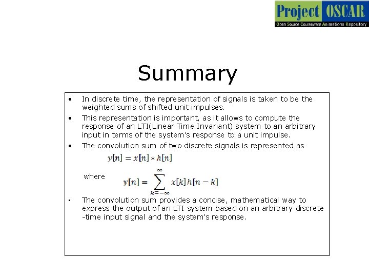
Summary • • • In discrete time, the representation of signals is taken to be the weighted sums of shifted unit impulses. This representation is important, as it allows to compute the response of an LTI(Linear Time Invariant) system to an arbitrary input in terms of the system’s response to a unit impulse. The convolution sum of two discrete signals is represented as where • The convolution sum provides a concise, mathematical way to express the output of an LTI system based on an arbitrary discrete -time input signal and the system‘s response.