Discrete and Recursive Models Eberhard O Voit Integrative

Discrete and Recursive Models Eberhard O. Voit Integrative Core Problem Solving with Models October 2011

Overarching Challenges of Modeling in Biology Map reality into a diagram Map diagram into symbolic equations Convert symbolic equations into functional symbolic equations Convert functional symbolic equations into parameterized equations The rest is comparatively straightforward!

So far: mostly ODEs Why? 1. Time is continuous (we believe) 2. It’s easier to describe instantaneous change than long-term trends 3. ODEs have many nice properties 4. Because of all that, there is a lot of software Why look for anything else? 1. Some things hard to represent (stochastic, spatial, delay effects, …) 2. Some processes are naturally discrete (at least in important aspects)

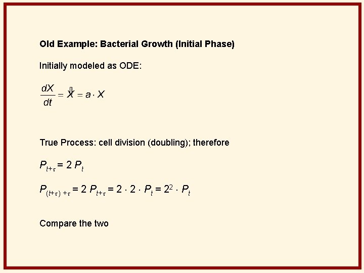
Old Example: Bacterial Growth (Initial Phase) Initially modeled as ODE: True Process: cell division (doubling); therefore Pt+t = 2 Pt P(t+t ) +t = 2 Pt+t = 2 2 Pt = 22 Pt Compare the two

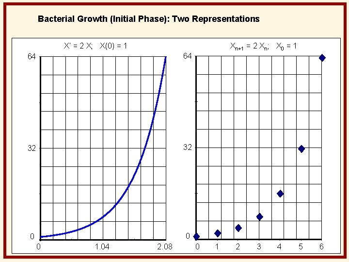
Bacterial Growth (Initial Phase): Two Representations X’ = 2 X; X(0) = 1 Xn+1 = 2 Xn; X 0 = 1 64 64 32 32 0 0 0 1. 04 2. 08 0 1 2 3 4 5 6

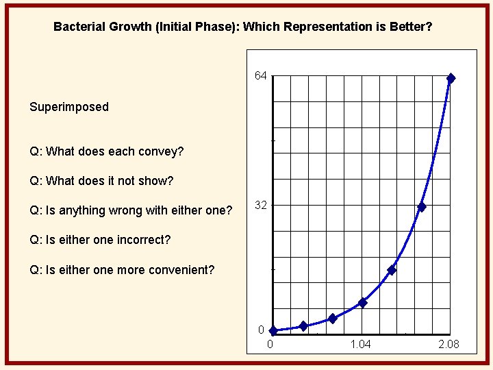
Bacterial Growth (Initial Phase): Which Representation is Better? 64 Superimposed Q: What does each convey? Q: What does it not show? Q: Is anything wrong with either one? 32 Q: Is either one incorrect? Q: Is either one more convenient? 0 0 1. 04 2. 08

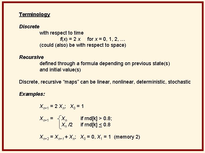
Terminology Discrete with respect to time f(x) = 2 x for x = 0, 1, 2, … (could (also) be with respect to space) Recursive defined through a formula depending on previous state(s) and initial value(s) Discrete, recursive “maps” can be linear, nonlinear, deterministic, stochastic Examples: Xn+1 = 2 Xn; X 0 = 1 Xn+1 = Xn Xn /2 if rnd[k] > 0. 8; if rnd[k] < 0. 8 Xn+2 = Xn+1 + Xn; X 0 = 0, X 1 = 1 (memory 2)

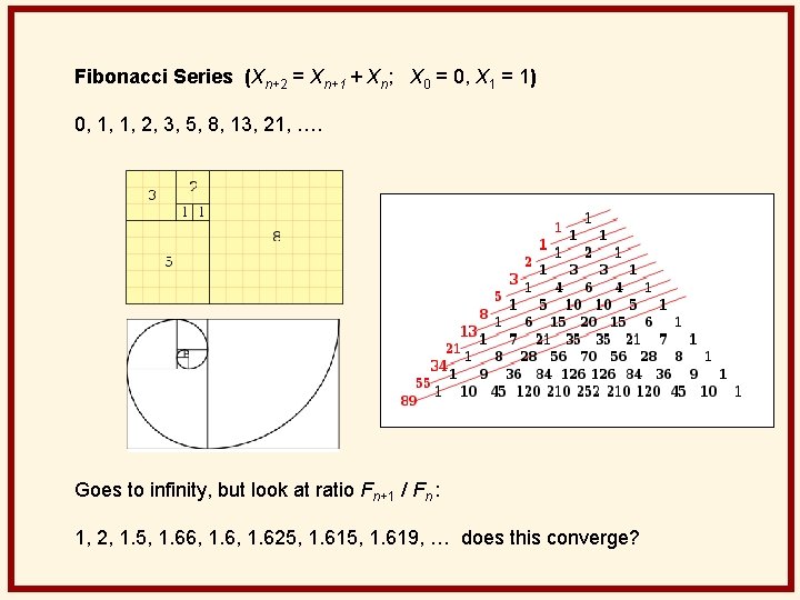
Fibonacci Series (Xn+2 = Xn+1 + Xn; X 0 = 0, X 1 = 1) 0, 1, 1, 2, 3, 5, 8, 13, 21, …. Goes to infinity, but look at ratio Fn+1 / Fn : 1, 2, 1. 5, 1. 66, 1. 625, 1. 619, … does this converge?

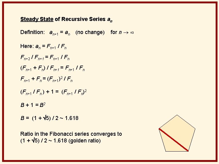
Steady State of Recursive Series an Definition: an+1 = an (no change) for n Here: an = Fn+1 / Fn Fn+2 / Fn+1 = Fn+1 / Fn (Fn+1 + Fn) / Fn+1 = Fn+1 / Fn Fn+1 + Fn = (Fn+1)2 / Fn (Fn+1 / Fn ) + 1 = (Fn+1 / Fn)2 B + 1 = B 2 B = (1 + 5) / 2 ~ 1. 618 Ratio in the Fibonacci series converges to (1 + 5) / 2 ~ 1. 618 (golden ratio)

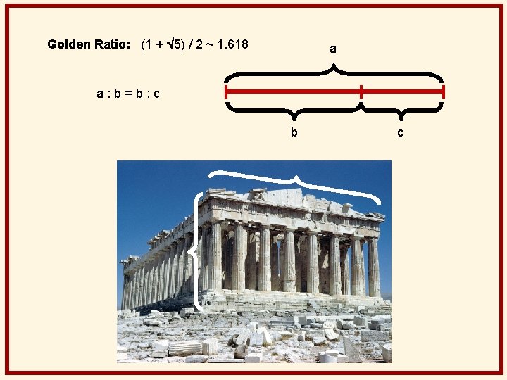
Golden Ratio: (1 + 5) / 2 ~ 1. 618 a a: b=b: c b c

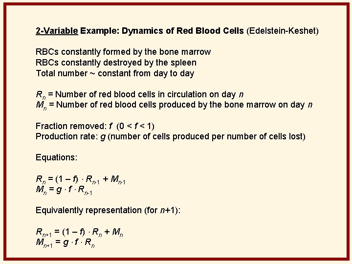
2 -Variable Example: Dynamics of Red Blood Cells (Edelstein-Keshet) RBCs constantly formed by the bone marrow RBCs constantly destroyed by the spleen Total number ~ constant from day to day Rn = Number of red blood cells in circulation on day n Mn = Number of red blood cells produced by the bone marrow on day n Fraction removed: f (0 < f < 1) Production rate: g (number of cells produced per number of cells lost) Equations: Rn = (1 – f) Rn-1 + Mn-1 Mn = g f Rn-1 Equivalently representation (for n+1): Rn+1 = (1 – f) Rn + Mn Mn+1 = g f Rn

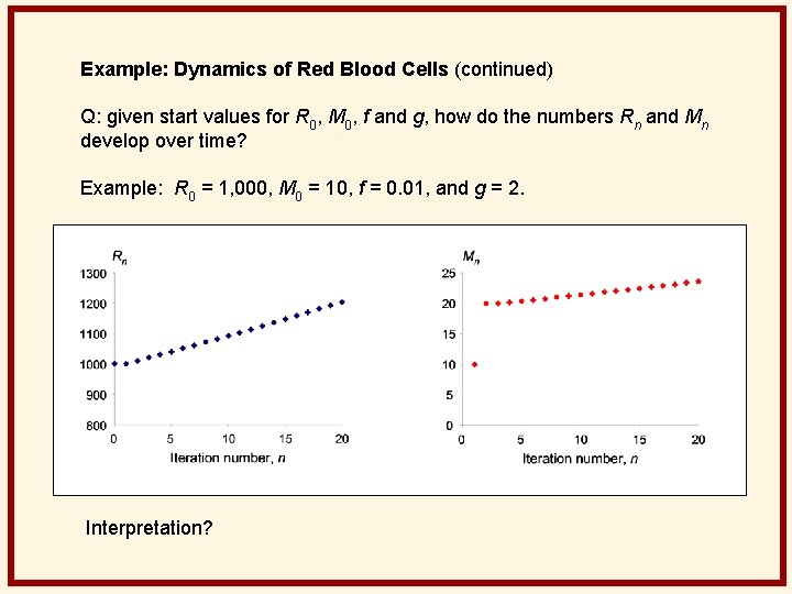
Example: Dynamics of Red Blood Cells (continued) Q: given start values for R 0, M 0, f and g, how do the numbers Rn and Mn develop over time? Example: R 0 = 1, 000, M 0 = 10, f = 0. 01, and g = 2. Interpretation?

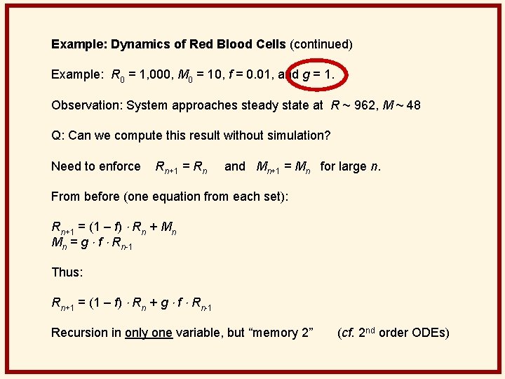
Example: Dynamics of Red Blood Cells (continued) Example: R 0 = 1, 000, M 0 = 10, f = 0. 01, and g = 1. Observation: System approaches steady state at R ~ 962, M ~ 48 Q: Can we compute this result without simulation? Need to enforce Rn+1 = Rn and Mn+1 = Mn for large n. From before (one equation from each set): Rn+1 = (1 – f) Rn + Mn Mn = g f Rn-1 Thus: Rn+1 = (1 – f) Rn + g f Rn-1 Recursion in only one variable, but “memory 2” (cf. 2 nd order ODEs)

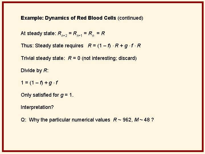
Example: Dynamics of Red Blood Cells (continued) At steady state: Rn+2 = Rn+1 = Rn = R Thus: Steady state requires R = (1 – f) R + g f R Trivial steady state: R = 0 (not interesting; discard) Divide by R: 1 = (1 – f) + g f Only satisfied for g = 1. Interpretation? Q: Why the particular numerical values R ~ 962, M ~ 48 ?

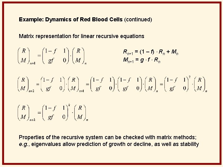
Example: Dynamics of Red Blood Cells (continued) Matrix representation for linear recursive equations Rn+1 = (1 – f) Rn + Mn Mn+1 = g f Rn Properties of the recursive system can be checked with matrix methods; e. g. , eigenvalues allow prediction of growth or decline, as well as stability

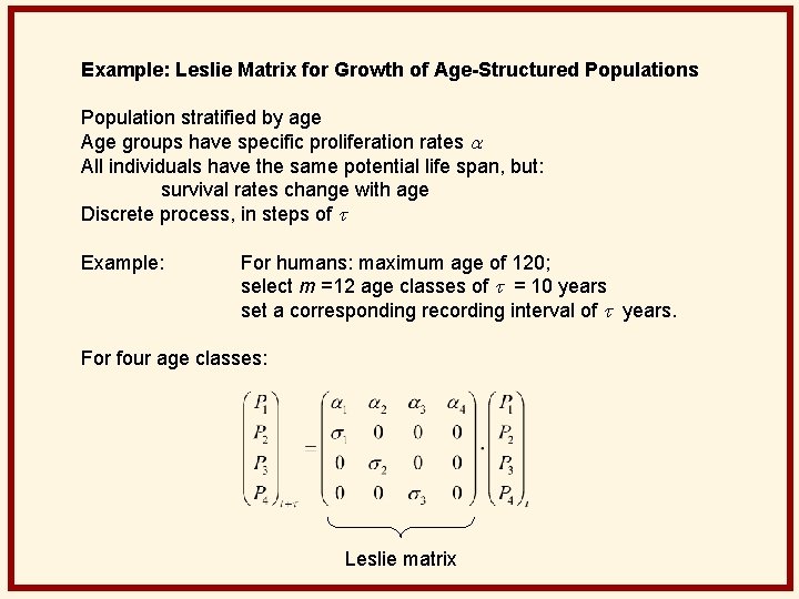
Example: Leslie Matrix for Growth of Age-Structured Populations Population stratified by age Age groups have specific proliferation rates a All individuals have the same potential life span, but: survival rates change with age Discrete process, in steps of t Example: For humans: maximum age of 120; select m =12 age classes of t = 10 years set a corresponding recording interval of t years. For four age classes: Leslie matrix

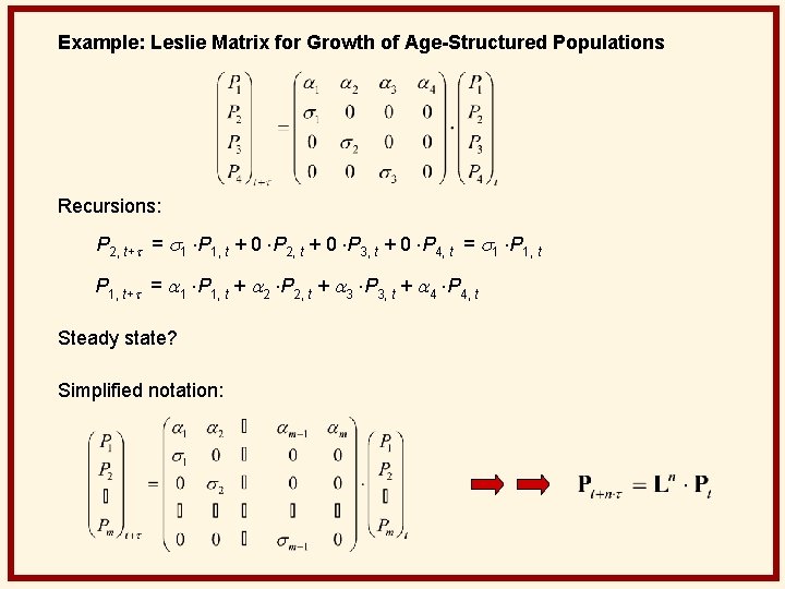
Example: Leslie Matrix for Growth of Age-Structured Populations Recursions: P 2, t+t = s 1 P 1, t + 0 P 2, t + 0 P 3, t + 0 P 4, t = s 1 P 1, t+t = a 1 P 1, t + a 2 P 2, t + a 3 P 3, t + a 4 P 4, t Steady state? Simplified notation:

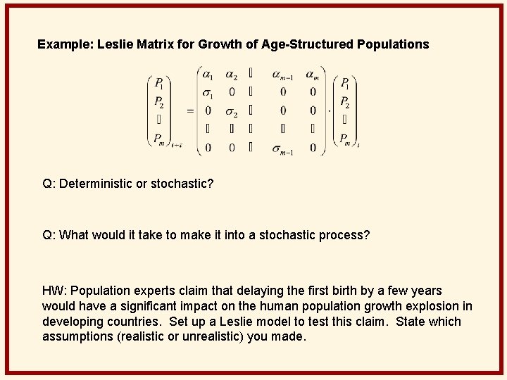
Example: Leslie Matrix for Growth of Age-Structured Populations Q: Deterministic or stochastic? Q: What would it take to make it into a stochastic process? HW: Population experts claim that delaying the first birth by a few years would have a significant impact on the human population growth explosion in developing countries. Set up a Leslie model to test this claim. State which assumptions (realistic or unrealistic) you made.

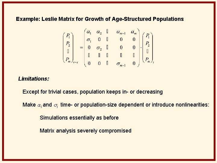
Example: Leslie Matrix for Growth of Age-Structured Populations Limitations: Except for trivial cases, population keeps in- or decreasing Make ai and si time- or population-size dependent or introduce nonlinearities: Simulations essentially as before Matrix analysis severely compromised

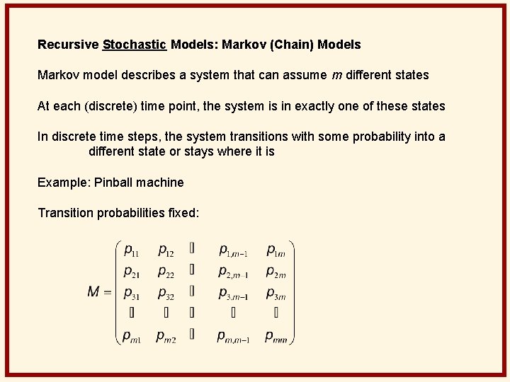
Recursive Stochastic Models: Markov (Chain) Models Markov model describes a system that can assume m different states At each (discrete) time point, the system is in exactly one of these states In discrete time steps, the system transitions with some probability into a different state or stays where it is Example: Pinball machine Transition probabilities fixed:

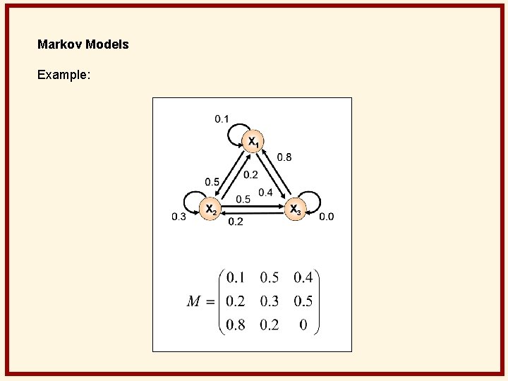
Markov Models Example:

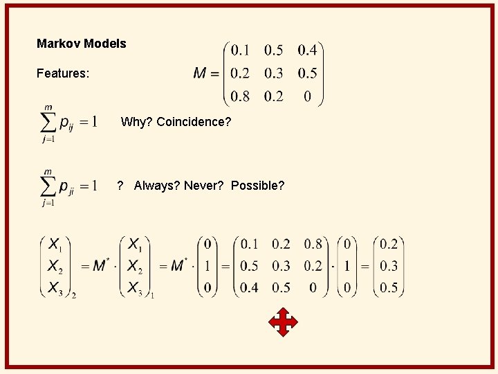
Markov Models Features: Why? Coincidence? ? Always? Never? Possible?

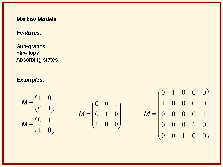
Markov Models Features: Sub-graphs Flip-flops Absorbing states Examples:

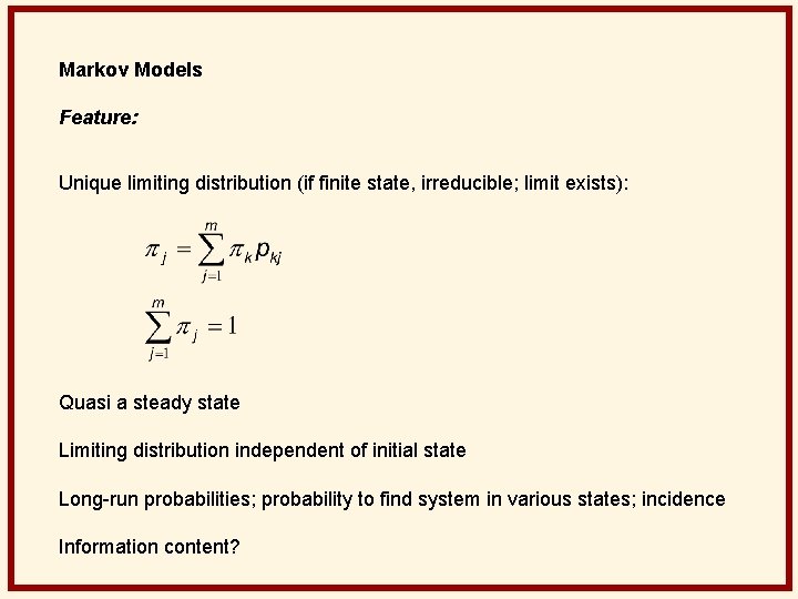
Markov Models Feature: Unique limiting distribution (if finite state, irreducible; limit exists): Quasi a steady state Limiting distribution independent of initial state Long-run probabilities; probability to find system in various states; incidence Information content?

Discrete Nonlinear Systems The sky is the limit! Just one example: Logistic map Pt+1 = r Pt (1– Pt) Name from logistic growth: B’ = r B – r/K B^2 Q: Similarity? Differences? P 0 (0, 1); r (0, 4)

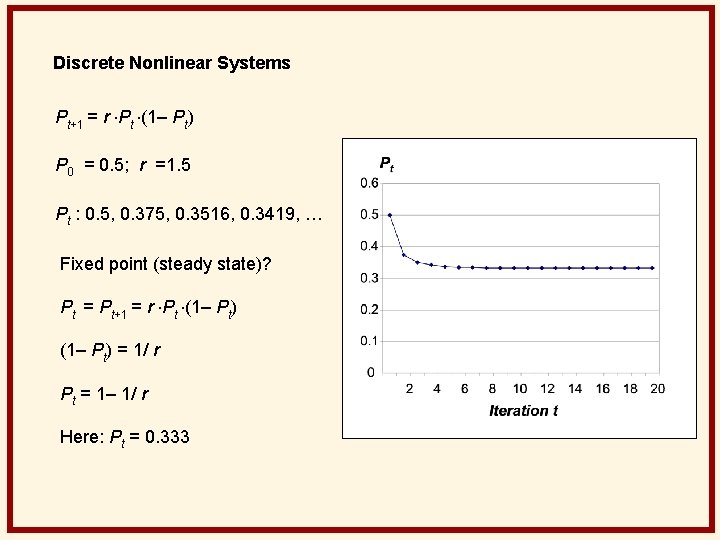
Discrete Nonlinear Systems Pt+1 = r Pt (1– Pt) P 0 = 0. 5; r =1. 5 Pt : 0. 5, 0. 375, 0. 3516, 0. 3419, … Fixed point (steady state)? Pt = Pt+1 = r Pt (1– Pt) = 1/ r Pt = 1– 1/ r Here: Pt = 0. 333

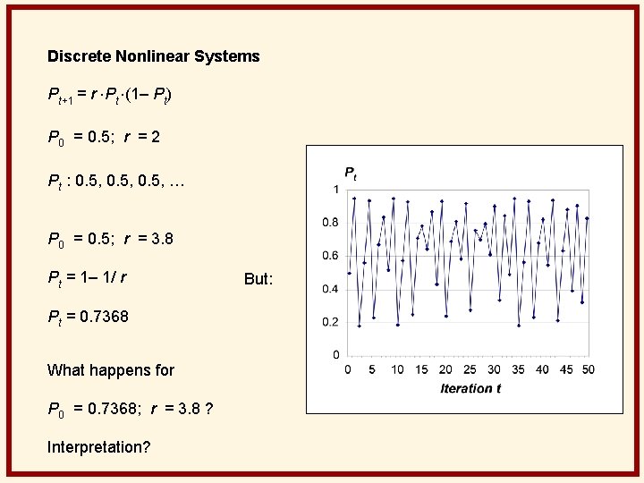
Discrete Nonlinear Systems Pt+1 = r Pt (1– Pt) P 0 = 0. 5; r = 2 Pt : 0. 5, … P 0 = 0. 5; r = 3. 8 Pt = 1– 1/ r Pt = 0. 7368 What happens for P 0 = 0. 7368; r = 3. 8 ? Interpretation? But:

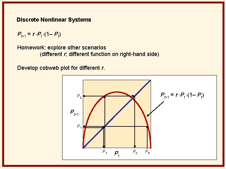
Discrete Nonlinear Systems Pt+1 = r Pt (1– Pt) Homework: explore other scenarios (different r; different function on right-hand side) Develop cobweb plot for different r. Pt+1 = r Pt (1– Pt) P 2 Pt+1 P 1 Pt P 2 P 0

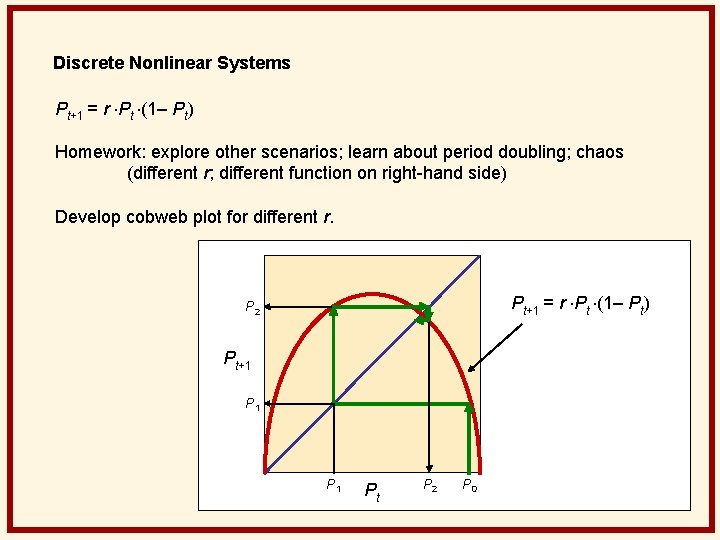
Discrete Nonlinear Systems Pt+1 = r Pt (1– Pt) Homework: explore other scenarios; learn about period doubling; chaos (different r; different function on right-hand side) Develop cobweb plot for different r. Pt+1 = r Pt (1– Pt) P 2 Pt+1 P 1 Pt P 2 P 0

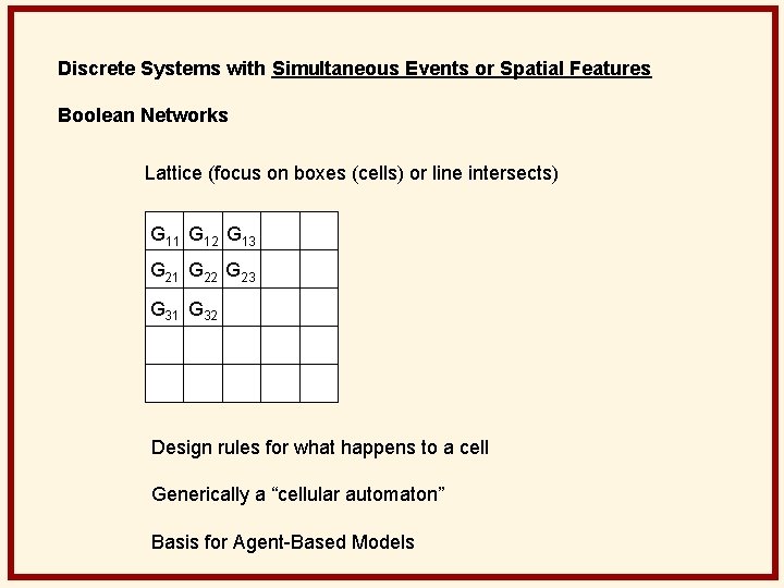
Discrete Systems with Simultaneous Events or Spatial Features Boolean Networks Lattice (focus on boxes (cells) or line intersects) G 11 G 12 G 13 G 21 G 22 G 23 G 31 G 32 Design rules for what happens to a cell Generically a “cellular automaton” Basis for Agent-Based Models

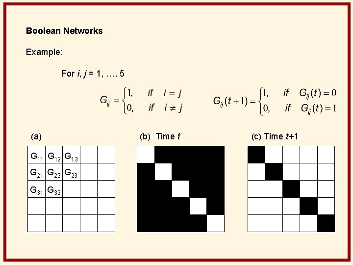
Boolean Networks Example: For i, j = 1, …, 5 (a) G 11 G 12 G 13 G 21 G 22 G 23 G 31 G 32 (b) Time t (c) Time t+1

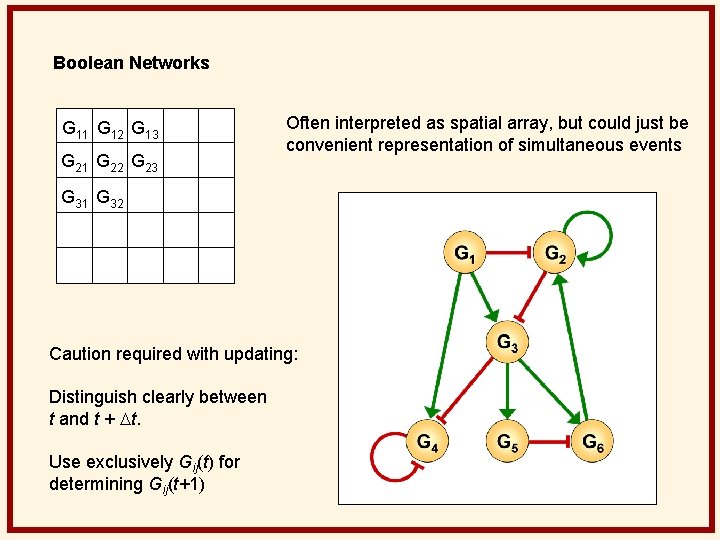
Boolean Networks G 11 G 12 G 13 G 21 G 22 G 23 Often interpreted as spatial array, but could just be convenient representation of simultaneous events G 31 G 32 Caution required with updating: Distinguish clearly between t and t + Dt. Use exclusively Gij(t) for determining Gij(t+1)

Boolean Networks Features: No real size limitation No principle limitation on complexity (not just functions, but rules) On-Off may be replaced by gradation (e. g. , 1 through 10) Usually no memory, but could be defined Can be made stochastic Can exhibit stable states, absorbing states, oscillations Chaos possible? Simulations easy; mathematical analysis complicated Refs: Stuart Kauffman: The Origins of Order (1993) John Conway: Game of Life (1970)

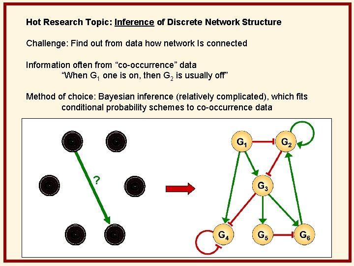
Hot Research Topic: Inference of Discrete Network Structure Challenge: Find out from data how network Is connected Information often from “co-occurrence” data “When G 1 one is on, then G 2 is usually off” Method of choice: Bayesian inference (relatively complicated), which fits conditional probability schemes to co-occurrence data G 1 G 2 ? G 6 G 5 G 3 G 4