Discovering the Intrinsic Cardinality and Dimensionality of Time

Discovering the Intrinsic Cardinality and Dimensionality of Time Series using MDL Bing Hu Thanawin Rakthanmanon Yuan Hao Scott Evans 1 Stefano Lonardi Eamonn Keogh {bhu 002, rakthant, yhao 002}@ucr. edu, 1 evans@ge. com, {stelo, eamonn}@cs. ucr. edu Department of Computer Science & Engineering University of California, Riverside 1 GE Global Research

Outline • Introduction • Modeling of MDL • Application Examples All the figures in this slides can be generated by running our code. All the data can be downloaded from the paper webpage

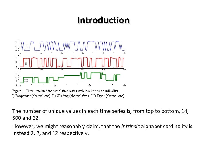
Introduction Figure 1. Three unrelated industrial time series with low intrinsic cardinality. I) Evaporator (channel one). II) Winding (channel five). III) Dryer (channel one). The number of unique values in each time series is, from top to bottom, 14, 500 and 62. However, we might reasonably claim, that the intrinsic alphabet cardinality is instead 2, 2, and 12 respectively.

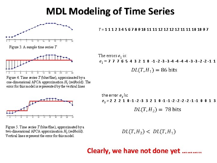
MDL Modeling of Time Series T = 1 1 1 2 3 4 5 6 7 8 9 10 11 11 12 12 11 11 10 10 9 7 Figure 3. A sample time series T The errors e 1 is: e 1 = 7 7 7 6 5 4 3 2 1 0 -1 -2 -3 -3 -4 -4 -3 -3 -2 -2 -1 1 Figure 4. Time series T (blue/fine), approximated by a one-dimensional APCA approximation H 1 (red/bold). The error for this model is represented by the vertical lines the error e 2 is: e 2 = 2 2 2 1 0 -1 -2 -3 3 2 1 0 -1 -1 -2 -2 -1 -1 0 0 1 3 Figure 5. Time series T (blue/fine), approximated by a two-dimensional APCA approximation H 2 (red/bold). Vertical lines represent the error for this model. Clearly, we have not done yet ………. .

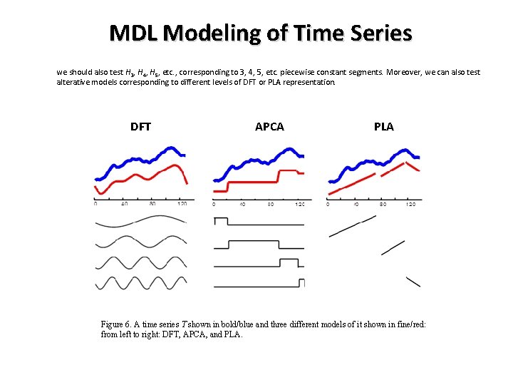
MDL Modeling of Time Series we should also test H 3, H 4, H 5, etc. , corresponding to 3, 4, 5, etc. piecewise constant segments. Moreover, we can also test alterative models corresponding to different levels of DFT or PLA representation. DFT APCA PLA Figure 6. A time series T shown in bold/blue and three different models of it shown in fine/red: from left to right: DFT, APCA, and PLA.

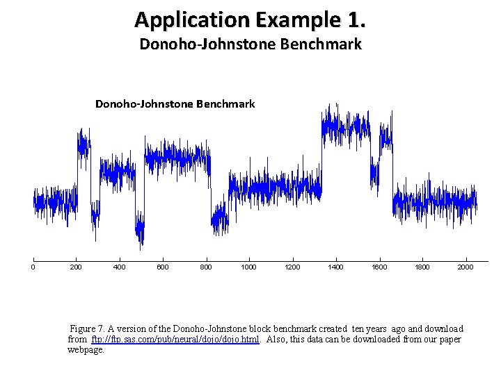
Application Example 1. Donoho-Johnstone Benchmark 0 200 400 600 800 1000 1200 1400 1600 1800 2000 Figure 7. A version of the Donoho-Johnstone block benchmark created ten years ago and download from ftp: //ftp. sas. com/pub/neural/dojo. html. Also, this data can be downloaded from our paper webpage.

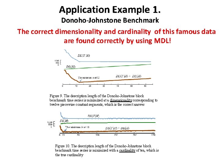
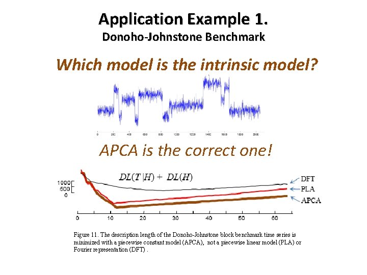
Application Example 1. Donoho-Johnstone Benchmark The correct dimensionality and cardinality of this famous data are found correctly by using MDL! Figure 9. The description length of the Donoho-Johnstone block benchmark time series is minimized at a dimensionality corresponding to twelve piecewise constant segments, which is the correct answer Figure 10. The description length of the Donoho-Johnstone block benchmark time series is minimized with a cardinality of ten, which is the true cardinality

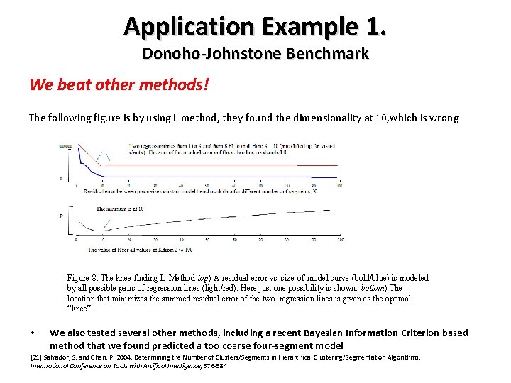
Application Example 1. Donoho-Johnstone Benchmark We beat other methods! The following figure is by using L method, they found the dimensionality at 10, which is wrong Figure 8. The knee finding L-Method top) A residual error vs. size-of-model curve (bold/blue) is modeled by all possible pairs of regression lines (light/red). Here just one possibility is shown. bottom) The location that minimizes the summed residual error of the two regression lines is given as the optimal “knee”. • We also tested several other methods, including a recent Bayesian Information Criterion based method that we found predicted a too coarse four-segment model [21] Salvador, S. and Chan, P. 2004. Determining the Number of Clusters/Segments in Hierarchical Clustering/Segmentation Algorithms. International Conference on Tools with Artifical Intelligence, 576 -584

Application Example 1. Donoho-Johnstone Benchmark Which model is the intrinsic model? APCA is the correct one! Figure 11. The description length of the Donoho-Johnstone block benchmark time series is minimized with a piecewise constant model (APCA), not a piecewise linear model (PLA) or Fourier representation (DFT).

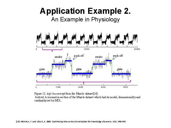
Application Example 2. An Example in Physiology Figure 12. top) An excerpt from the Muscle dataset[16]. bottom) A zoomed-in section of the Muscle dataset which had its model, dimensionality and cardinality set by MDL [16] Mörchen, F. and Ultsch, A. 2005. Optimizing time series discretization for knowledge discovery. KDD, 660 -665

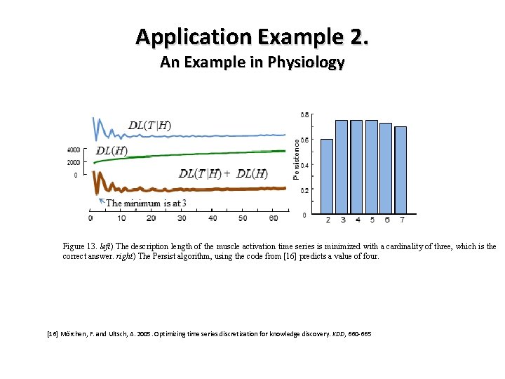
Application Example 2. An Example in Physiology Figure 13. left) The description length of the muscle activation time series is minimized with a cardinality of three, which is the correct answer. right) The Persist algorithm, using the code from [16] predicts a value of four. [16] Mörchen, F. and Ultsch, A. 2005. Optimizing time series discretization for knowledge discovery. KDD, 660 -665

Application Example 2. An Example in Physiology • The dataset is from paper [16]Mörchen, F. and Ultsch, A. 2005. Optimizing time series discretization for knowledge discovery. KDD, 660 -665 We download the dataset from the author’ webpage http: //www. mybytes. de/persist. php You can also download the data from our paper webpage.

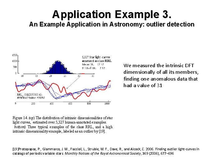
Application Example 3. An Example Application in Astronomy: outlier detection We measured the intrinsic DFT dimensionally of all its members, finding one anomalous data that had a value of 31 Figure 14. top) The distribution of intrinsic dimensionalities of star light curves, estimated over 5, 327 human-annotated examples. bottom) Three typical examples of the class RRL, and a high intrinsic dimensionality example, labeled as an outlier by [19]Protopapas, P. , Giammarco, J. M. , Faccioli, L. , Struble, M. F. , Dave, R. , and Alcock, C. 2006. Finding outlier light-curves in catalogs of periodic variable stars. Monthly Notices of the Royal Astronomical Society, 369 (2006), 677– 696

Application Example 3. An Example Application in Astronomy: outlier detection The star light curve data can be downloaded from the paper webpage.

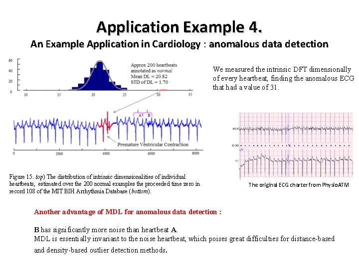
Application Example 4. An Example Application in Cardiology : Cardiology anomalous data detection We measured the intrinsic DFT dimensionally of every heartbeat, finding the anomalous ECG that had a value of 31. Figure 15. top) The distribution of intrinsic dimensionalities of individual heartbeats, estimated over the 200 normal examples the proceeded time zero in record 108 of the MIT BIH Arrhythmia Database (bottom). The original ECG charter from Physio. ATM Another advantage of MDL for anomalous data detection : B has significantly more noise than heartbeat A. MDL is essentially invariant to the noise heartbeat, which poises great difficulties for distance-based and density-based outlier detection methods.

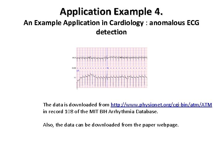
Application Example 4. An Example Application in Cardiology : Cardiology anomalous ECG detection The data is downloaded from http: //www. physionet. org/cgi-bin/atm/ATM in record 108 of the MIT BIH Arrhythmia Database. Also, the data can be downloaded from the paper webpage.