Discovering Significant Association Rules Dean L Zeller Kent

Discovering Significant Association Rules Dean L. Zeller Kent State University CS 73015 – Data Mining Dr. Ruomin Jin “If you … beat this [cop] long enough, he’ll tell you he started the … Chicago Fire. Now that don’t necessarily make it so!” -- Nice Guy Eddie Reservoir Dogs (1995) Discovering Significant Association Rules

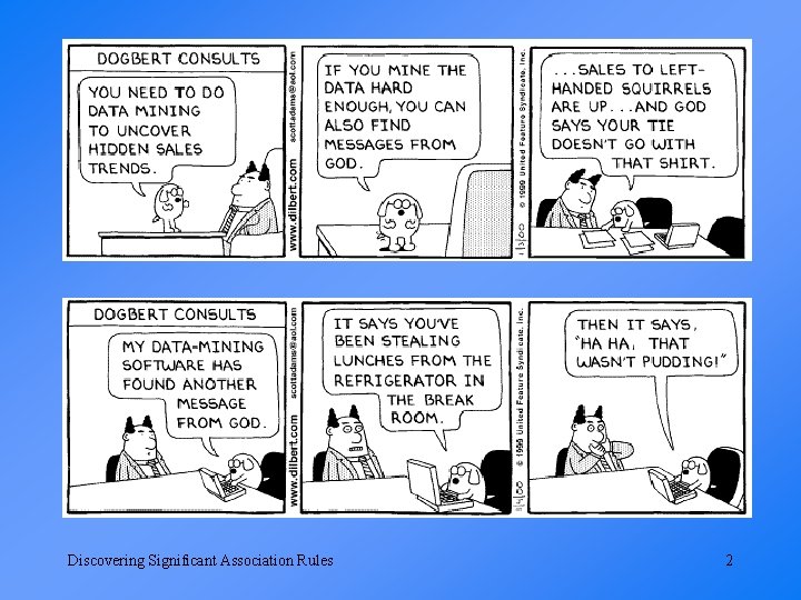
Discovering Significant Association Rules 2

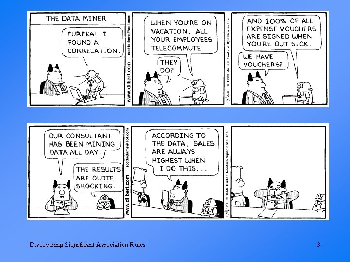
Discovering Significant Association Rules 3

Introduction • • • Association Rules Causation vs. Association Uses of Association Rules True and False Discoveries Measures of Interestingness “We, the members of the data mining community, are doing a serious disservice to ourselves, as well as to the communities we seek to serve, if we present sets of ‘discoveries’ to our clients of which the majority are spurious. ” -- Geoffrey Webb Discovering Significant Association Rules 4

Association Rules • Association rule mining is hot new area of programming. • Statistical measures must be taken to quickly and efficiently evaluate the “interestingness” of a rule (i. e. represent non-trivial correlations). • Avoid false discoveries Discovering Significant Association Rules 5

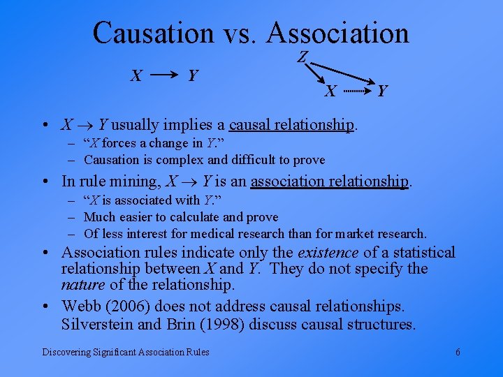
Causation vs. Association Z X Y • X Y usually implies a causal relationship. – “X forces a change in Y. ” – Causation is complex and difficult to prove • In rule mining, X Y is an association relationship. – “X is associated with Y. ” – Much easier to calculate and prove – Of less interest for medical research than for market research. • Association rules indicate only the existence of a statistical relationship between X and Y. They do not specify the nature of the relationship. • Webb (2006) does not address causal relationships. Silverstein and Brin (1998) discuss causal structures. Discovering Significant Association Rules 6

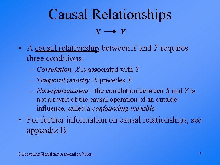
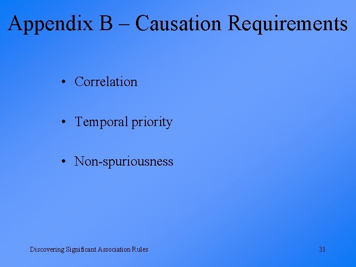
Causal Relationships X Y • A causal relationship between X and Y requires three conditions: – Correlation: X is associated with Y – Temporal priority: X precedes Y – Non-spuriousness: the correlation between X and Y is not a result of the causal operation of an outside influence, called a confounding variable. • For further information on causal relationships, see appendix B. Discovering Significant Association Rules 7

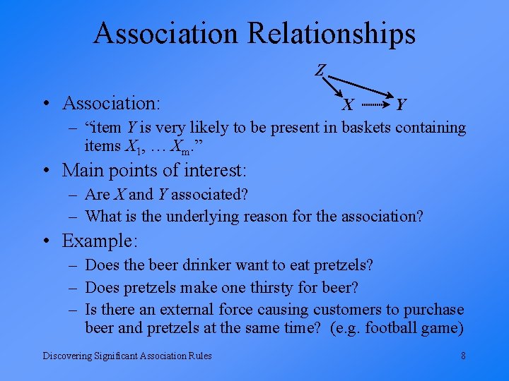
Association Relationships Z • Association: X Y – “item Y is very likely to be present in baskets containing items X 1, … Xm. ” • Main points of interest: – Are X and Y associated? – What is the underlying reason for the association? • Example: – Does the beer drinker want to eat pretzels? – Does pretzels make one thirsty for beer? – Is there an external force causing customers to purchase beer and pretzels at the same time? (e. g. football game) Discovering Significant Association Rules 8

True vs. False Discoveries • On some real-world problems there is potential for all ‘discoveries’ to be false unless appropriate safeguards are employed. • Create definitions, requirements, and formulas for “true” and “false” discoveries based on the data. • Specify in terms of arbitrary statistical hypothesis tests. • Provide strict control over the risk of false discoveries. Discovering Significant Association Rules 9

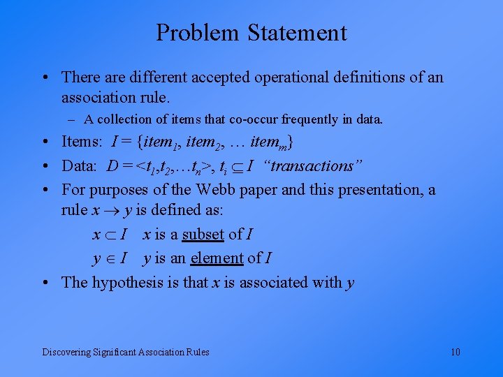
Problem Statement • There are different accepted operational definitions of an association rule. – A collection of items that co-occur frequently in data. • Items: I = {item 1, item 2, … itemm} • Data: D = <t 1, t 2, …tn>, ti I “transactions” • For purposes of the Webb paper and this presentation, a rule x y is defined as: x I x is a subset of I y is an element of I • The hypothesis is that x is associated with y Discovering Significant Association Rules 10

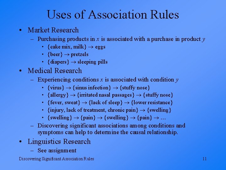
Uses of Association Rules • Market Research – Purchasing products in x is associated with a purchase in product y • {cake mix, milk} eggs • {beer} pretzels • {diapers} sleeping pills • Medical Research – Experiencing conditions x is associated with condition y • • • {virus} {sinus infection} {stuffy nose} {allergy} {irritated nasal passages} {stuffy nose} {fever, sweat} {lack of sleep} {lower resistance} {injury, lack of treatment, chronic pain} {swelling} {pain} … – Discovering significant associations among conditions and symptoms can help to determine the causal relationship. • Linguistics Research – See assignment Discovering Significant Association Rules 11

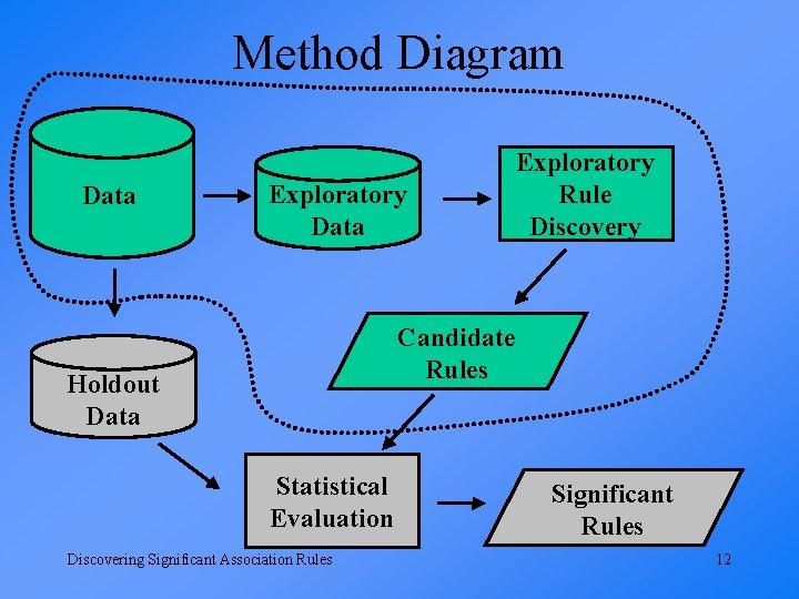
Method Diagram Data Exploratory Rule Discovery Candidate Rules Holdout Data Statistical Evaluation Discovering Significant Association Rules Significant Rules 12

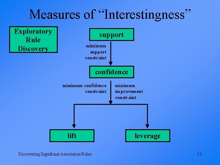
Measures of “Interestingness” Exploratory Rule Discovery support minimum support constraint confidence minimum confidence constraint lift Discovering Significant Association Rules minimum improvement constraint leverage 13

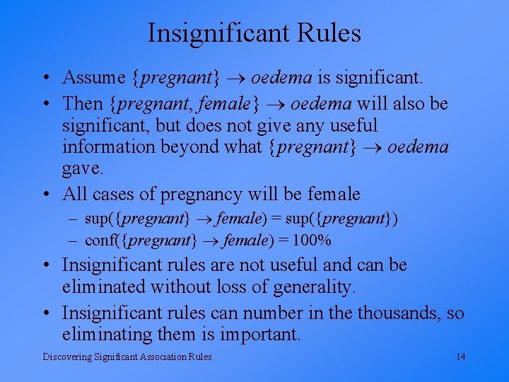
Insignificant Rules • Assume {pregnant} oedema is significant. • Then {pregnant, female} oedema will also be significant, but does not give any useful information beyond what {pregnant} oedema gave. • All cases of pregnancy will be female – sup({pregnant} female) = sup({pregnant}) – conf({pregnant} female) = 100% • Insignificant rules are not useful and can be eliminated without loss of generality. • Insignificant rules can number in the thousands, so eliminating them is important. Discovering Significant Association Rules 14

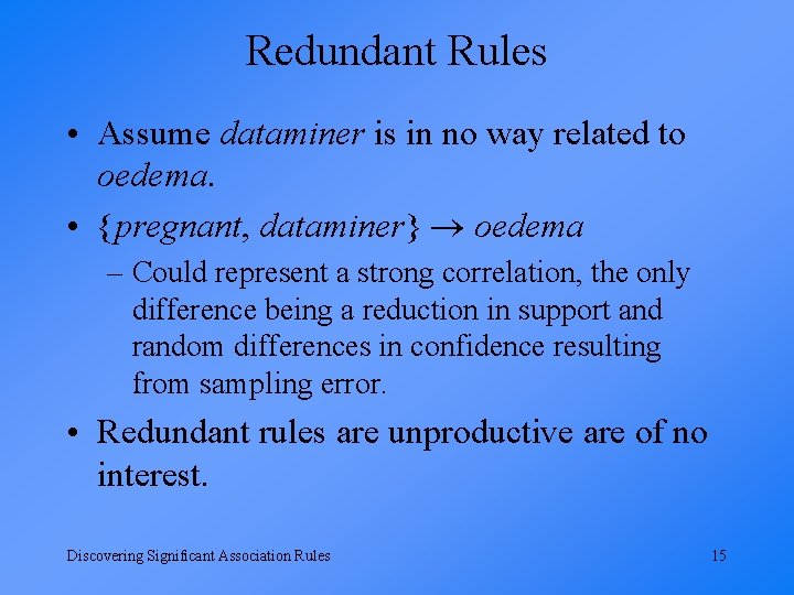
Redundant Rules • Assume dataminer is in no way related to oedema. • {pregnant, dataminer} oedema – Could represent a strong correlation, the only difference being a reduction in support and random differences in confidence resulting from sampling error. • Redundant rules are unproductive are of no interest. Discovering Significant Association Rules 15

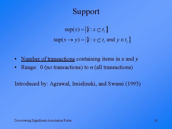
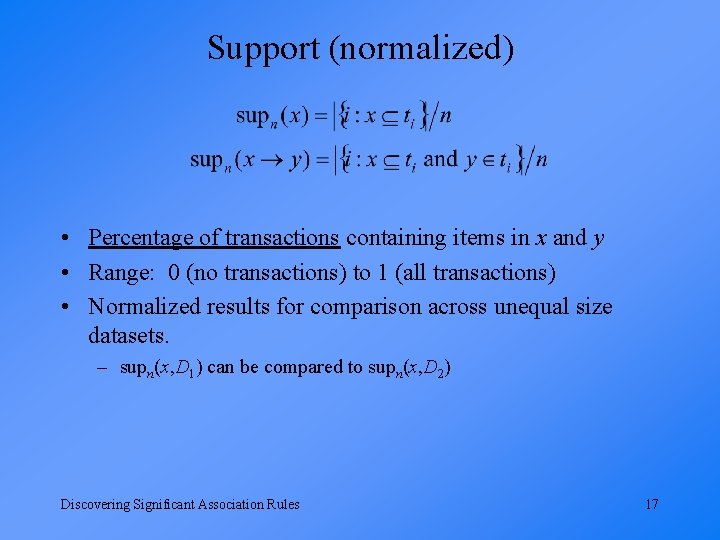
Support • Number of transactions containing items in x and y • Range: 0 (no transactions) to n (all transactions) Introduced by: Agrawal, Imielinski, and Swami (1993) Discovering Significant Association Rules 16

Support (normalized) • Percentage of transactions containing items in x and y • Range: 0 (no transactions) to 1 (all transactions) • Normalized results for comparison across unequal size datasets. – supn(x, D 1) can be compared to supn(x, D 2) Discovering Significant Association Rules 17

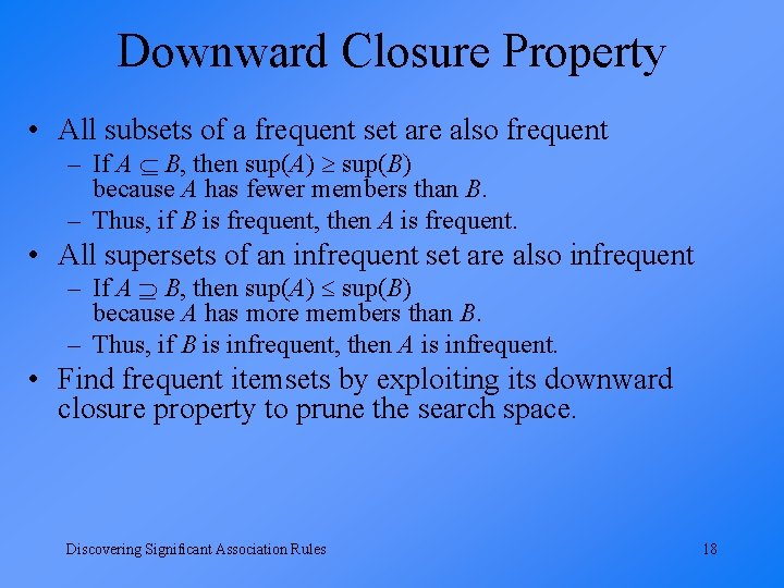
Downward Closure Property • All subsets of a frequent set are also frequent – If A B, then sup(A) sup(B) because A has fewer members than B. – Thus, if B is frequent, then A is frequent. • All supersets of an infrequent set are also infrequent – If A B, then sup(A) sup(B) because A has more members than B. – Thus, if B is infrequent, then A is infrequent. • Find frequent itemsets by exploiting its downward closure property to prune the search space. Discovering Significant Association Rules 18

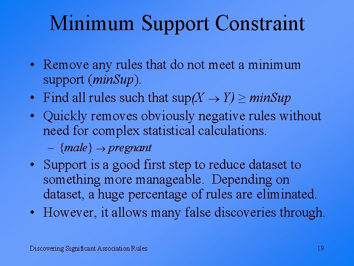
Minimum Support Constraint • Remove any rules that do not meet a minimum support (min. Sup). • Find all rules such that sup(X Y) ≥ min. Sup • Quickly removes obviously negative rules without need for complex statistical calculations. – {male} pregnant • Support is a good first step to reduce dataset to something more manageable. Depending on dataset, a huge percentage of rules are eliminated. • However, it allows many false discoveries through. Discovering Significant Association Rules 19

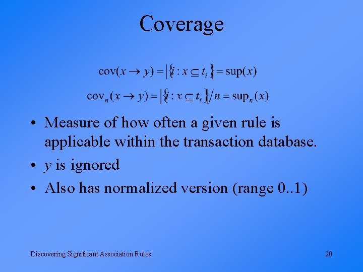
Coverage • Measure of how often a given rule is applicable within the transaction database. • y is ignored • Also has normalized version (range 0. . 1) Discovering Significant Association Rules 20

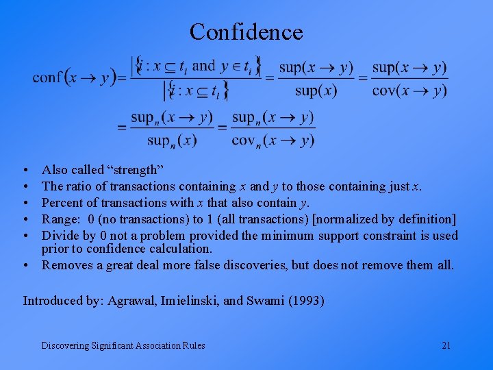
Confidence • • • Also called “strength” The ratio of transactions containing x and y to those containing just x. Percent of transactions with x that also contain y. Range: 0 (no transactions) to 1 (all transactions) [normalized by definition] Divide by 0 not a problem provided the minimum support constraint is used prior to confidence calculation. • Removes a great deal more false discoveries, but does not remove them all. Introduced by: Agrawal, Imielinski, and Swami (1993) Discovering Significant Association Rules 21

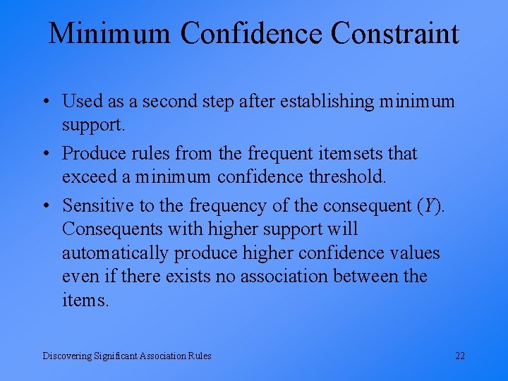
Minimum Confidence Constraint • Used as a second step after establishing minimum support. • Produce rules from the frequent itemsets that exceed a minimum confidence threshold. • Sensitive to the frequency of the consequent (Y). Consequents with higher support will automatically produce higher confidence values even if there exists no association between the items. Discovering Significant Association Rules 22

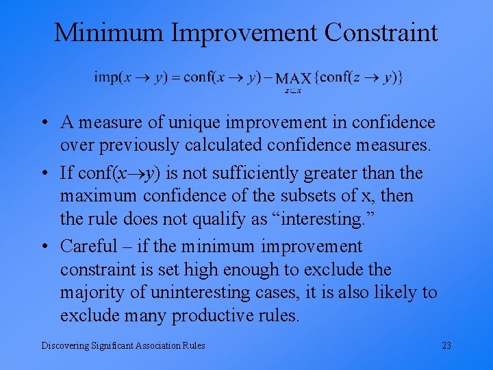
Minimum Improvement Constraint • A measure of unique improvement in confidence over previously calculated confidence measures. • If conf(x y) is not sufficiently greater than the maximum confidence of the subsets of x, then the rule does not qualify as “interesting. ” • Careful – if the minimum improvement constraint is set high enough to exclude the majority of uninteresting cases, it is also likely to exclude many productive rules. Discovering Significant Association Rules 23

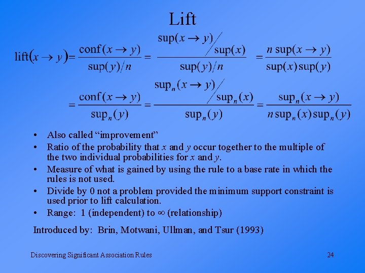
Lift • Also called “improvement” • Ratio of the probability that x and y occur together to the multiple of the two individual probabilities for x and y. • Measure of what is gained by using the rule to a base rate in which the rules is not used. • Divide by 0 not a problem provided the minimum support constraint is used prior to lift calculation. • Range: 1 (independent) to (relationship) Introduced by: Brin, Motwani, Ullman, and Tsur (1993) Discovering Significant Association Rules 24

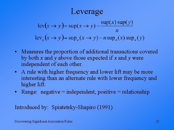
Leverage • Measures the proportion of additional transactions covered by both x and y above those expected if x and y were independent of each other. • A rule with higher frequency and lower lift may be more interesting than an alternate rule with lower frequency and higher lift. • Range: negative = independent, positive = relationship Introduced by: Spiatetsky-Shapiro (1991) Discovering Significant Association Rules 25

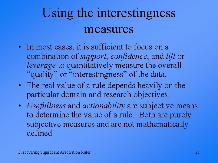
Using the interestingness measures • In most cases, it is sufficient to focus on a combination of support, confidence, and lift or leverage to quantitatively measure the overall “quality” or “interestingness” of the data. • The real value of a rule depends heavily on the particular domain and research objectives. • Usefullness and actionability are subjective means to determine the value of a rule. Both are purely subjective measures and are not mathematically defined. Discovering Significant Association Rules 26

References • Agrawal R. , Imielinski, T. , and Swami, A. “Mining associations between sets of items in large databases. ” Proceedings of the ACM SIGMOD International Conference on Management of Data (ACM SIGMOD ’ 93), pages 207 -216, Washington DC, May 1993. • Brin, S. , Motwani, R. , Ullman, J. D. , and Tsur, S. “Dynamic itemset counting and implication rules for market basket data” Proceedings of the ACM SIGMOD International Conference on Management of Data (ACM SIGMOD ’ 97), pages 207216, Washington DC, May 1993. • Silverstein, C. , Brin, S. , Motwani, R. , Ullman, J. “Scalable Techniques for Mining Causal Structures. ” Proceedings of the 24 th VLDB Conference, pages 594 -605, New York City, 1998. • Spiatetsky-Shapiro, G. , “Discovery, analysis, and presentation of strong rules. ” Knowledge Discovery in Databases, pages 229 -248, 1991. • Webb, G. I. “Discovering Significant Rules. ”KDD ‘ 06, pages 434 -443, Philadelphia, Pennsylvania, August 2006. • Zeller, R. A. Personal correspondence, October 2006. Discovering Significant Association Rules 27

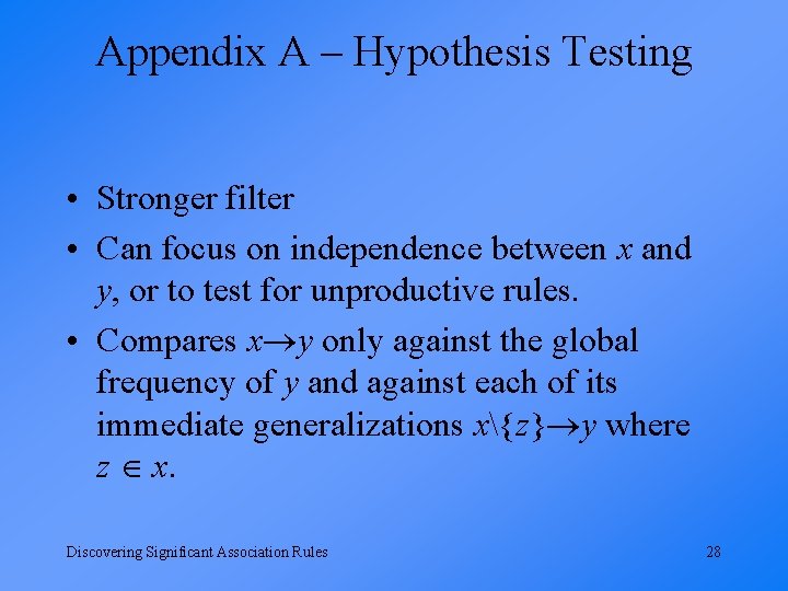
Appendix A – Hypothesis Testing • Stronger filter • Can focus on independence between x and y, or to test for unproductive rules. • Compares x y only against the global frequency of y and against each of its immediate generalizations x{z} y where z x. Discovering Significant Association Rules 28

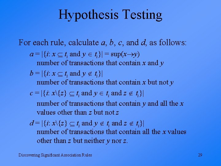
Hypothesis Testing For each rule, calculate a, b, c, and d, as follows: a = |{i: x ti and y ti}| = sup(x y) number of transactions that contain x and y b = |{i: x ti and y ti}| number of transactions that contain x but not y c = |{i: x{z} ti and y ti and z ti}| number of transactions that contain y and all the x values other than z but not z d = |{i: x{z} ti and y ti and z ti}| number of transactions that contain all the x values other than z but neither y nor z. Discovering Significant Association Rules 29

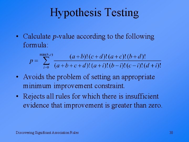
Hypothesis Testing • Calculate p-value according to the following formula: • Avoids the problem of setting an appropriate minimum improvement constraint. • Rejects all rules for which there is insufficient evidence that improvement is greater than zero. Discovering Significant Association Rules 30

Appendix B – Causation Requirements • Correlation • Temporal priority • Non-spuriousness Discovering Significant Association Rules 31

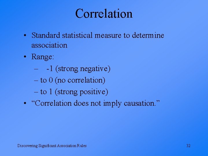
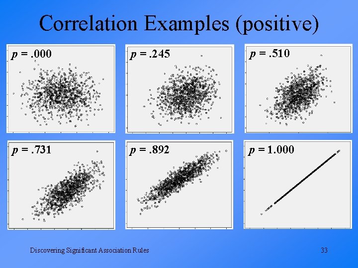
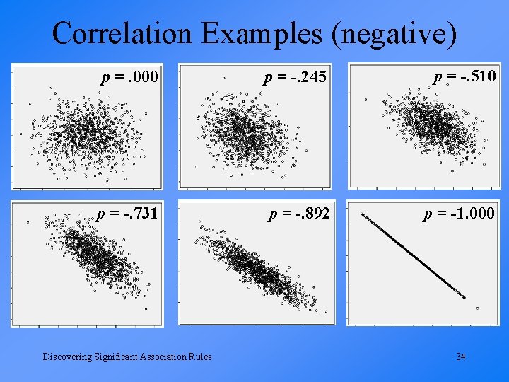
Correlation • Standard statistical measure to determine association • Range: – -1 (strong negative) – to 0 (no correlation) – to 1 (strong positive) • “Correlation does not imply causation. ” Discovering Significant Association Rules 32

Correlation Examples (positive) p =. 000 p =. 245 p =. 510 p =. 731 p =. 892 p = 1. 000 Discovering Significant Association Rules 33

Correlation Examples (negative) p =. 000 p = -. 245 p = -. 510 p = -. 731 p = -. 892 p = -1. 000 Discovering Significant Association Rules 34

Temporal priority • X must precede Y. • Easy to measure in some cases. – “The fever occurred before the chicken pox formed. ” • Difficult to measure in others. – “She bought the milk before the eggs. ” • Impossible in some cases (e. g. anything male) • Simultaneous Reverse Causation – “Statistical magic” to justify that X causes Y and Y causes X at the same time. • Important note: the time of measurement is not necessarily the same as time of occurrence. Discovering Significant Association Rules 35

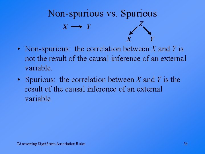
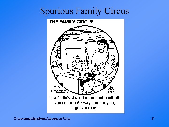
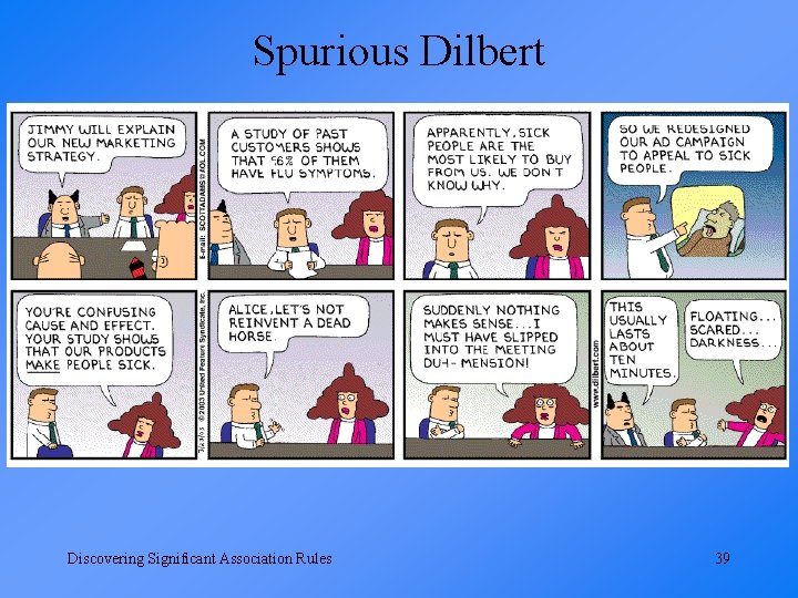
Non-spurious vs. Spurious X Z Y X Y • Non-spurious: the correlation between X and Y is not the result of the causal inference of an external variable. • Spurious: the correlation between X and Y is the result of the causal inference of an external variable. Discovering Significant Association Rules 36

Spurious Family Circus Discovering Significant Association Rules 37

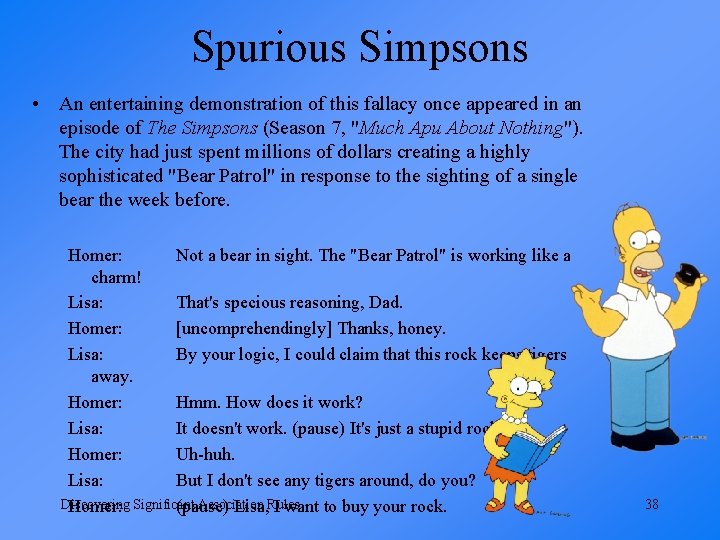
Spurious Simpsons • An entertaining demonstration of this fallacy once appeared in an episode of The Simpsons (Season 7, "Much Apu About Nothing"). The city had just spent millions of dollars creating a highly sophisticated "Bear Patrol" in response to the sighting of a single bear the week before. Homer: Not a bear in sight. The "Bear Patrol" is working like a charm! Lisa: That's specious reasoning, Dad. Homer: [uncomprehendingly] Thanks, honey. Lisa: By your logic, I could claim that this rock keeps tigers away. Homer: Hmm. How does it work? Lisa: It doesn't work. (pause) It's just a stupid rock! Homer: Uh-huh. Lisa: But I don't see any tigers around, do you? Discovering Association Homer: Significant (pause) Lisa, Rules I want to buy your rock. 38

Spurious Dilbert Discovering Significant Association Rules 39

Spurious Relationships • These are all known strong correlations. What is the actual cause of each? – ice-cream sales and drowning occurrences – number of firemen at a fire and dollar value of damage caused – college students having more sex get better grades – volume of beer purchased at Mardi Gras and volume of water in the Mississippi River – voters cause more auto-accidents than non-voters – depression causes loneliness vs. loneliness causes depression Discovering Significant Association Rules 40

Spurious Relationships • Sleeping with one's shoes on is strongly correlated with waking up with a headache. Therefore, sleeping with one's shoes on causes headache. The above example commits the correlation implies causation fallacy, as it prematurely concludes that sleeping with one's shoes on causes headache. A more plausible explanation is that both are caused by a third factor, in this case alcohol intoxication, which thereby gives rise to a correlation. • Young children who sleep with the light on are much more likely to develop myopia in later life. This result of a study at University of Pennsylvania Medical Center was published in the May 13, 1999, issue of Nature and received much coverage at the time in the popular press. However a later study at Ohio State University did not find any link between infants sleeping with the light on and developing myopia but did find a strong link between parental myopia and the development of child myopia and also noted that myopic parents were more likely to leave a light on in their children's bedroom. • Since the 1950 s, both the atmospheric CO 2 level and crime levels have increased sharply. Hence, atmospheric CO 2 causes crime. The above example arguably makes the mistake of prematurely concluding a causal relationship where the relationship between the variables, if any, is so complex it may be labeled coincidental. The two events have no simple relationship to each other beside the fact that they are occurring at the same time. • Not eating causes anorexia nervosa. Having the disease Anorexia Nervosa may be the cause of not eating. It is correct that not eating does cause anorexia nervosa, but it can also be claimed that having developed anorexia nervosa causes one not to eat. Empirical evidence would be necessary to make a causative statement. • Scientific research finds that people who use cannabis (A) have a higher prevalence of psychiatric disorders compared to those who do not (B). This particular correlation is sometimes used to support theory that the use of cannabis causes a psychiatric disorder (A is the cause of B). Although this may be possible, we cannot automatically discern a cause and effect relationship from research that has only determined people who use cannabis are more likely to develop a psychiatric disorder. From the same research, it can also be the case that (1. ) having the predisposition for a psychiatric disorder causes these individuals to use cannabis (B causes A), OR (2. )it may be the case that in the above study some unknown third factor (e. g. , poverty) is the actual cause for there being found a higher number of people (compared to the general public) who both use cannabis and who have been diagnosed as having a psychiatric disorder. Alternatively, it may be that the effects of cannabis are found more pleasurable by persons with certain psychiatric disorders. To assume that A causes B is tempting, but further scientific investigation of the type that can isolate extraneous variables is needed when research has only determined a statistical correlation. Source: Wikipedia Discovering Significant Association Rules 41