Discovering Cyclic Causal Models by Independent Components Analysis

Discovering Cyclic Causal Models by Independent Components Analysis Gustavo Lacerda Peter Spirtes Joseph Ramsey Patrik O. Hoyer

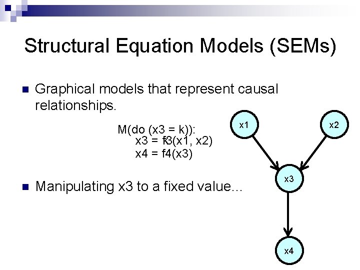
Structural Equation Models (SEMs) n Graphical models that represent causal relationships. M(do (x 3 = k)): M: x 3 = kf 3(x 1, x 2) x 4 = f 4(x 3) n x 1 Manipulating x 3 to a fixed value… x 2 x 3 x 4

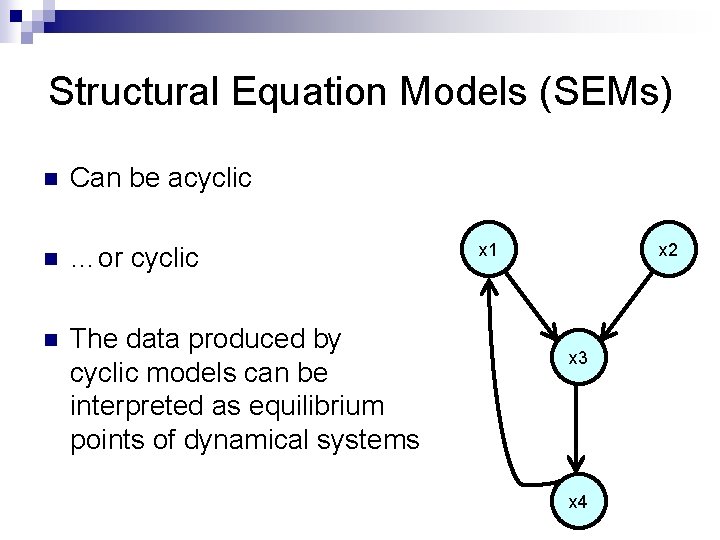
Structural Equation Models (SEMs) n Can be acyclic n …or cyclic n The data produced by cyclic models can be interpreted as equilibrium points of dynamical systems x 1 x 2 x 3 x 4

Linear Structural Equation Models (SEMs) (deterministic example) n The structural equations are linear n e. g. : x 3 = 1. 2 x 1 + 0. 9 x 2 - 3 x 4 = -5 x 3 + 1 n Each edge weight tells us the corresponding coefficient x 1 x 2 1. 2 0. 9 x 3 -5 x 4

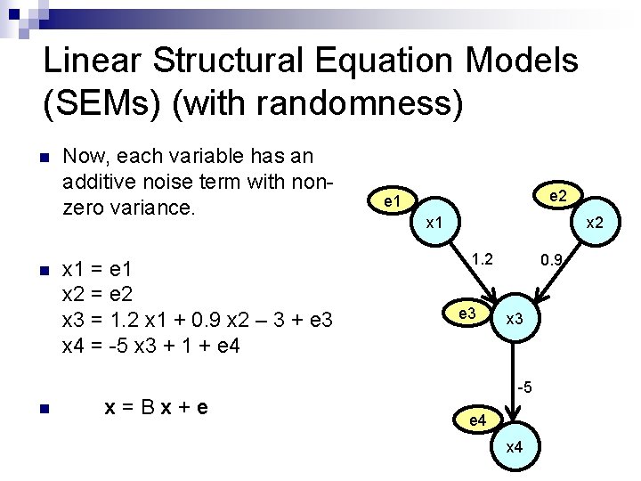
Linear Structural Equation Models (SEMs) (with randomness) n n n Now, each variable has an additive noise term with nonzero variance. x 1 = e 1 x 2 = e 2 x 3 = 1. 2 x 1 + 0. 9 x 2 – 3 + e 3 x 4 = -5 x 3 + 1 + e 4 x=Bx+e e 2 e 1 x 2 1. 2 e 3 0. 9 x 3 -5 e 4 x 4

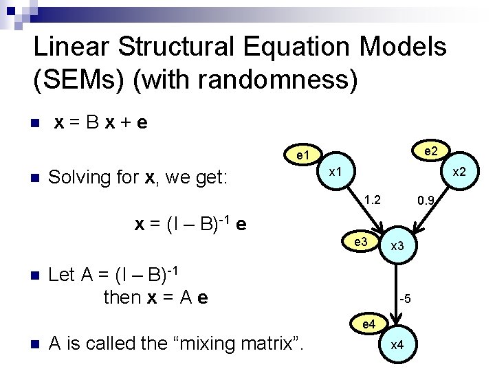
Linear Structural Equation Models (SEMs) (with randomness) n x=Bx+e e 2 e 1 n Solving for x, we get: x 1 x 2 1. 2 0. 9 x = (I – B)-1 e e 3 n Let A = (I – B)-1 then x = A e x 3 -5 e 4 n A is called the “mixing matrix”. x 4

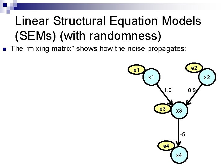
Linear Structural Equation Models (SEMs) (with randomness) n The “mixing matrix” shows how the noise propagates: e 2 e 1 x 2 1. 2 e 3 0. 9 x 3 -5 e 4 x 4

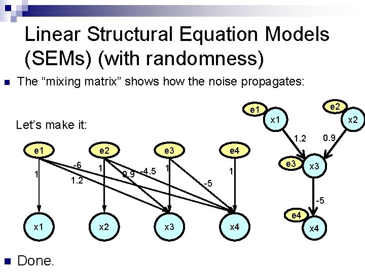
Linear Structural Equation Models (SEMs) (with randomness) n The “mixing matrix” shows how the noise propagates: e 2 e 1 x 1 Let’s make it: x 2 0. 9 1. 2 e 1 1 e 2 -6 1 1. 2 e 3 1 0. 9 -4. 5 e 4 1 e 3 x 3 -5 -5 e 4 x 1 n Done. x 2 x 3 x 4

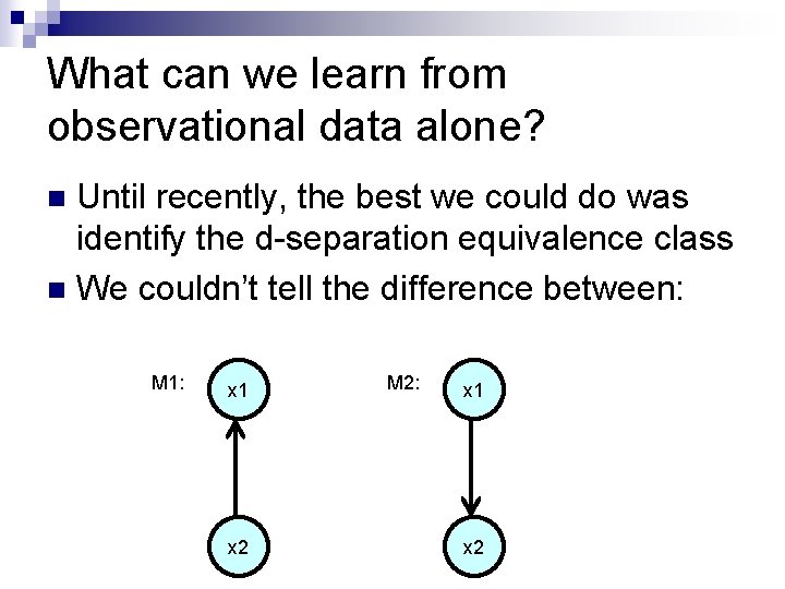
What can we learn from observational data alone? Until recently, the best we could do was identify the d-separation equivalence class n We couldn’t tell the difference between: n M 1: x 1 x 2 M 2: x 1 x 2

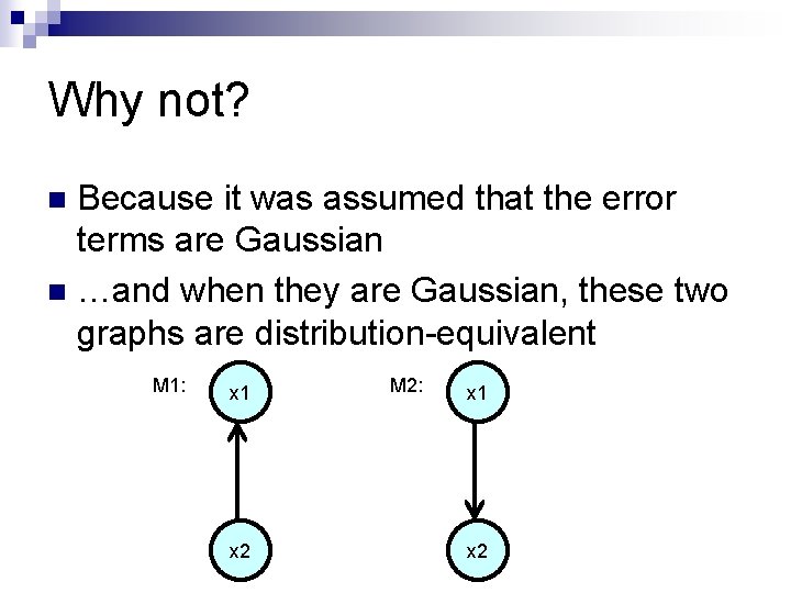
Why not? Because it was assumed that the error terms are Gaussian n …and when they are Gaussian, these two graphs are distribution-equivalent n M 1: x 1 x 2 M 2: x 1 x 2

Independent Components Analysis (ICA) n Cocktail party problem e 1 e 2 x=Ae x 1 n x 2 You want to get back the original signals, but all you have are the mixtures. What can you do?

Independent Components Analysis (ICA) n Cocktail party problem e 1 e 2 x=Ae x 1 x 2 n This equation has infinitely many solutions! For any invertible A, there is a solution! n But if you assume that the signals are independent, it is possible to estimate A and e from just x. n How?

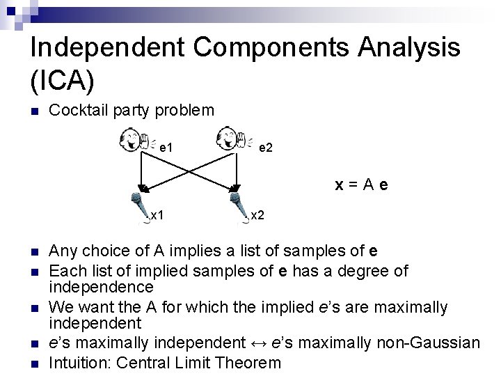
Independent Components Analysis (ICA) n Cocktail party problem e 1 e 2 x=Ae x 1 n n n x 2 Any choice of A implies a list of samples of e Each list of implied samples of e has a degree of independence We want the A for which the implied e’s are maximally independent e’s maximally independent ↔ e’s maximally non-Gaussian Intuition: Central Limit Theorem

Independent Components Analysis (ICA) n We don’t know which source signal is which, i. e. which is Alex and which is Bob n Scaling: when used with SEMs, the variance of each error term is confounded with its coefficients on each x.

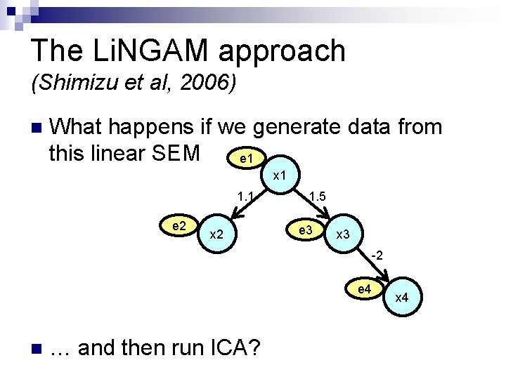
The Li. NGAM approach (Shimizu et al, 2006) n What happens if we generate data from this linear SEM e 1 x 1 1. 1 e 2 x 2 1. 5 e 3 x 3 -2 e 4 n … and then run ICA? x 4

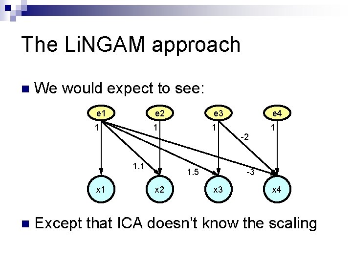
The Li. NGAM approach n We would expect to see: e 1 e 2 e 3 e 4 1 1 1. 1 x 1 n 1. 5 x 2 -2 -3 x 4 Except that ICA doesn’t know the scaling

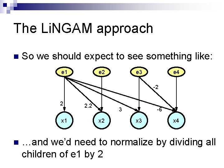
The Li. NGAM approach n So we should expect to see something like: e 1 e 2 e 3 e 4 -2 2 x 1 n 2. 2 3 x 2 -6 x 3 x 4 …and we’d need to normalize by dividing all children of e 1 by 2

The Li. NGAM approach n getting us: e 1 e 2 e 3 e 4 -2 1 x 1 n 1. 1 1. 5 x 2 -3 x 4 Except that ICA doesn’t know the order of the e’s, i. e. which e’s go with which x’s…

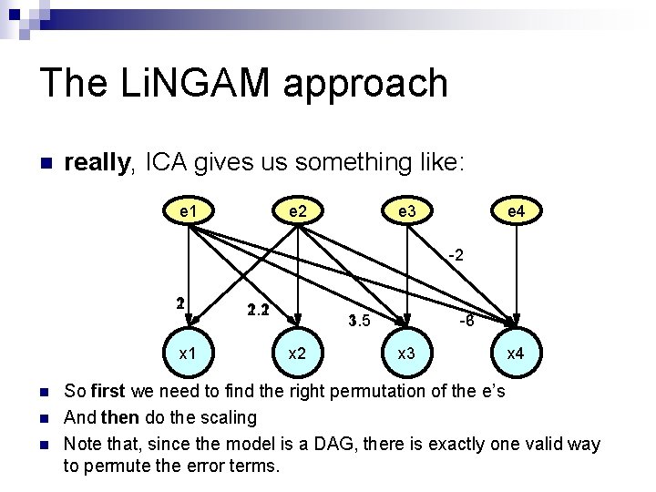
The Li. NGAM approach n really, ICA gives us something like: e… e 1 e… e 2 e… e 3 e… e 4 -2 2 1 x 1 n n n 2. 2 1. 1 3 1. 5 x 2 -6 -3 x 4 So first we need to find the right permutation of the e’s And then do the scaling Note that, since the model is a DAG, there is exactly one valid way to permute the error terms.

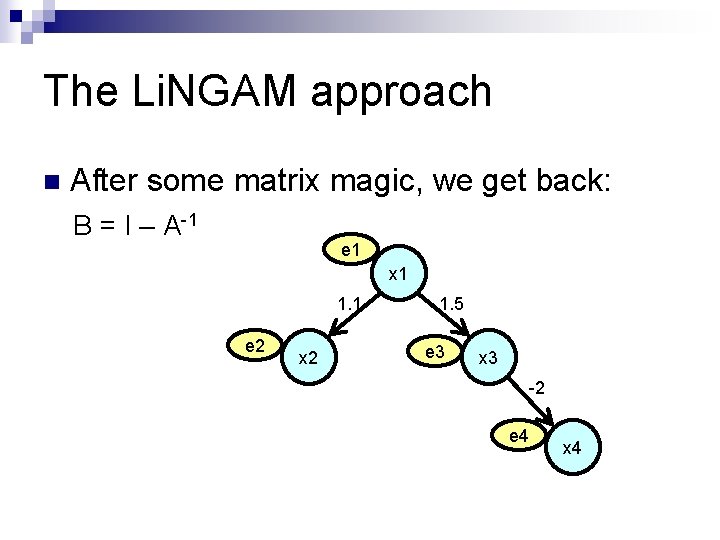
The Li. NGAM approach n After some matrix magic, we get back: B = I – A-1 e 1 x 1 1. 1 e 2 x 2 1. 5 e 3 x 3 -2 e 4 x 4

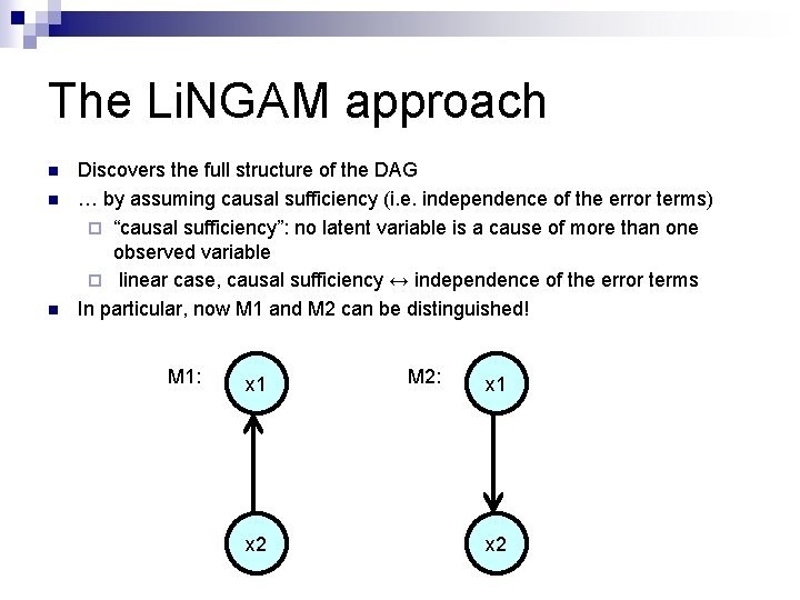
The Li. NGAM approach n n n Discovers the full structure of the DAG … by assuming causal sufficiency (i. e. independence of the error terms) ¨ “causal sufficiency”: no latent variable is a cause of more than one observed variable ¨ linear case, causal sufficiency ↔ independence of the error terms In particular, now M 1 and M 2 can be distinguished! M 1: x 1 x 2 M 2: x 1 x 2

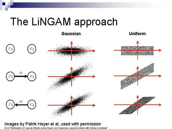
The Li. NGAM approach Gaussian Images by Patrik Hoyer et al, used with permission from “Estimation of causal effects using linear non-Gaussian causal models with hidden variables” Uniform

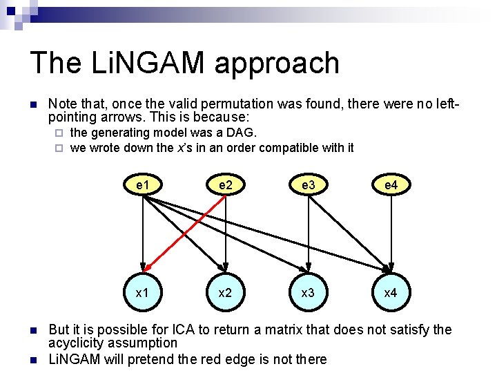
The Li. NGAM approach n Note that, once the valid permutation was found, there were no leftpointing arrows. This is because: ¨ ¨ n n the generating model was a DAG. we wrote down the x’s in an order compatible with it e 1 e 2 e 3 e 4 x 1 x 2 x 3 x 4 But it is possible for ICA to return a matrix that does not satisfy the acyclicity assumption Li. NGAM will pretend the red edge is not there

The Li. NGAM approach n n Li. NGAM cannot discover cyclic models… because: ¨ since it assumes the data was generated by a DAG, ¨ it searches for a single valid permutation n If we search for any number of valid permutations… then we can discover cyclic models too. That’s exactly what we did!

The Li. NG-DG approach n When the data looks acyclic, it works just like Li. NGAM, and returns a single model. n When the data looks cyclic, more than one permutation is considered valid. Thus, it returns a distribution-equivalent set containing more than one model. n “distribution-equivalent” means you can’t do better, at least without experimental data or further assumptions.

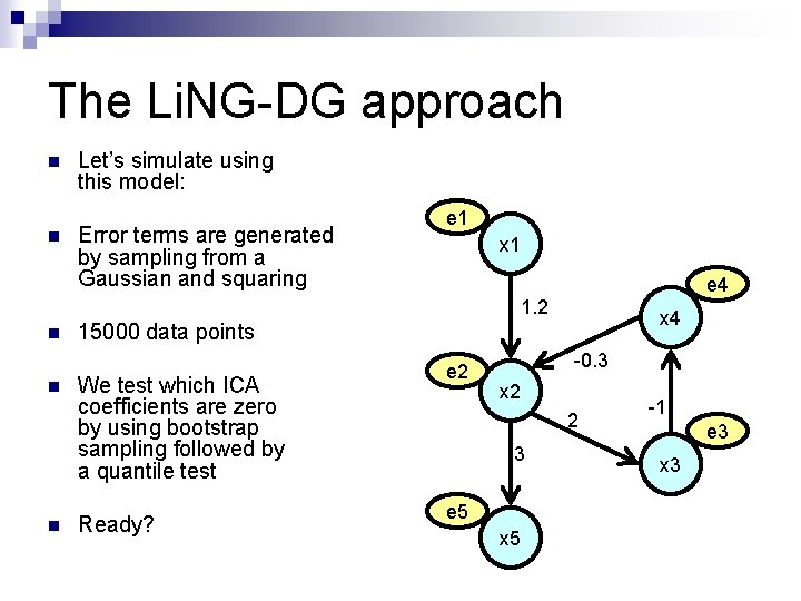
The Li. NG-DG approach n n Let’s simulate using this model: Error terms are generated by sampling from a Gaussian and squaring e 1 x 1 e 4 1. 2 n n n x 4 15000 data points We test which ICA coefficients are zero by using bootstrap sampling followed by a quantile test Ready? e 2 -0. 3 x 2 2 3 e 5 x 5 -1 e 3 x 3

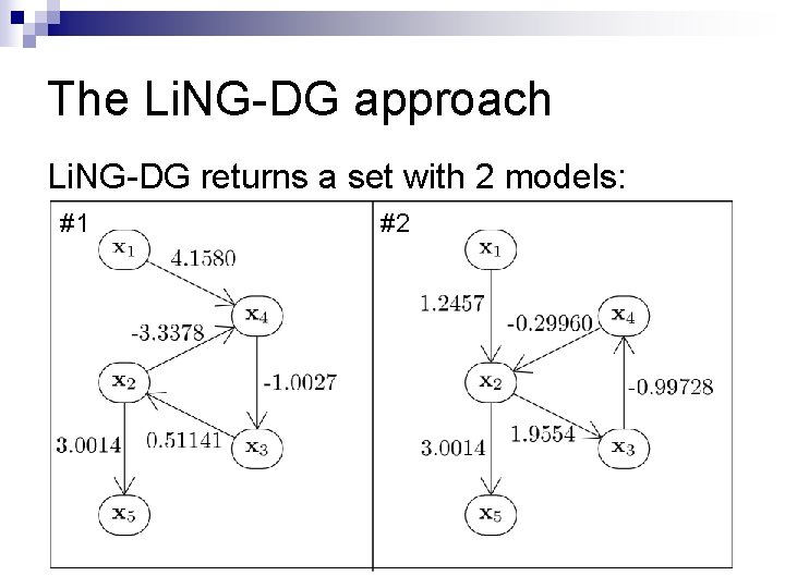
The Li. NG-DG approach Li. NG-DG returns a set with 2 models: #1 #2

Li. NG-DG + the stability assumption Note that only one of these models is stable. n If our data is a set of equilibria, then the true model must be stable. n n Under what conditions are we guaranteed to have a unique stable model?

Li. NG-DG + the stability assumption n Theorem: if the true model’s cycles don’t intersect, then only one model is stable. n For simple cycle models, cycle-products are inverted: c 1 = 1/c 2. So at least one cycle will be > 1 (in modulus) and thus unstable. each cycle works independently, and any valid permutation* will invert at least one cycle, creating an unstable model. n n *except for the identity permutation

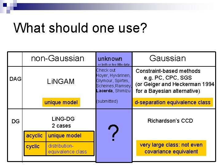
What should one use? non-Gaussian DAG Li. NGAM unique model Li. NG-DG 2 cases DG acyclic unique model cyclic distributionequivalence class unknown or both or too little data Gaussian Check out Hoyer, Hyvärinen, Glymour, Spirtes, Scheines, Ramsey, Lacerda, Shimizu Constraint-based methods e. g. PC, CPC, SGS (or Geiger and Heckerman 1994 for a Bayesian alternative) (submitted) d-separation equivalence class ? Richardson’s CCD very large class: not even covariance equivalent

UAI is due soon! Please send me your comments: gusl@cs. cmu. edu

Appendix 1: self-loops n Equilibrium equations usually correspond with the dynamical equations. n EXCEPT if a self-loop has coefficient 1, we will get the wrong structure, and the predicted results of intervention will be wrong! n self-loop coefficients are underdetermined. n Our stability results only hold if we assume no self-loops.

Appendix 2: search and pruning n Testing zeros: local vs non-local methods n To estimate the variance of the estimated coefficients, we use bootstrap sampling, carefully. n How to find row-permutations of W that have a zeroless diagonal: ¨ Acyclic: Hungarian algorithm ¨ General: k-best linear assignments, or constrained n. Rooks (put rooks on the non-zero entries)