
Disconnected Loop Subtraction Methods Suman Baral a c
Disconnected Loop Subtraction Methods Suman Baral a, c, Travis Whyte a, *, Walter Wilcox a and Ronald Morganb a. Department b. Department c. Everest of Physics, Baylor University, Waco, TX 76798 -7316, United States of Mathematics, Baylor University, Waco TX 76798 -7316, United States Institute of Science and Technology, Samakhusi Kathmandu, Nepal * Speaker Comp. Phys. Comm 241 (2019) 64 -79
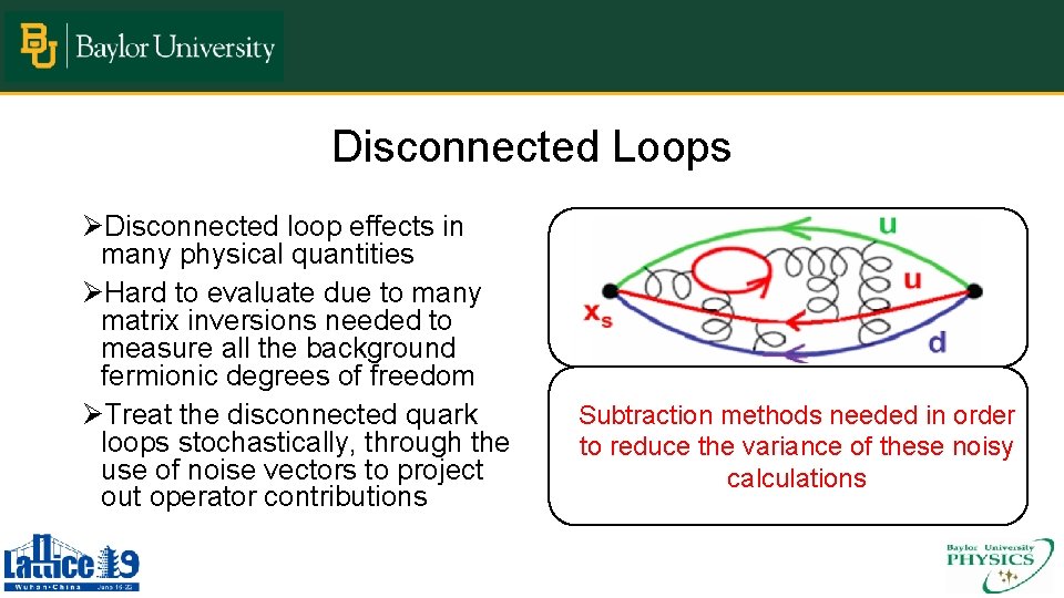
Disconnected Loops ØDisconnected loop effects in many physical quantities ØHard to evaluate due to many matrix inversions needed to measure all the background fermionic degrees of freedom ØTreat the disconnected quark loops stochastically, through the use of noise vectors to project out operator contributions Subtraction methods needed in order to reduce the variance of these noisy calculations
Noise Theory
Noise Theory
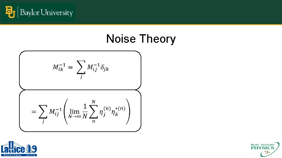
Noise Theory
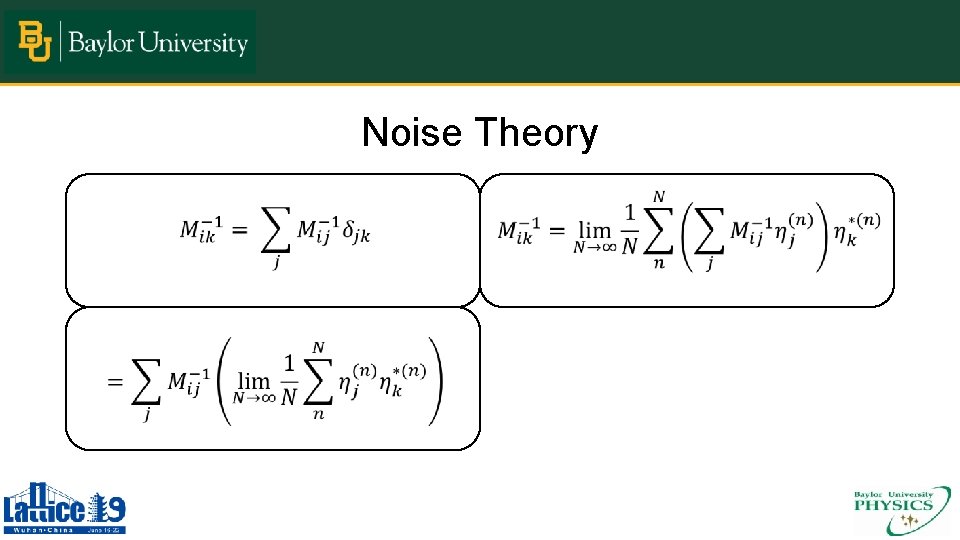
Noise Theory
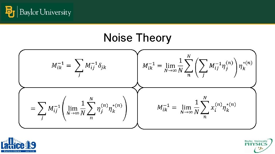
Noise Theory
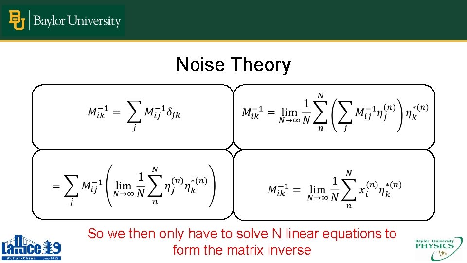
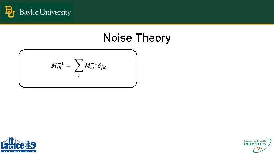
Noise Theory So we then only have to solve N linear equations to form the matrix inverse
Noise Subtraction
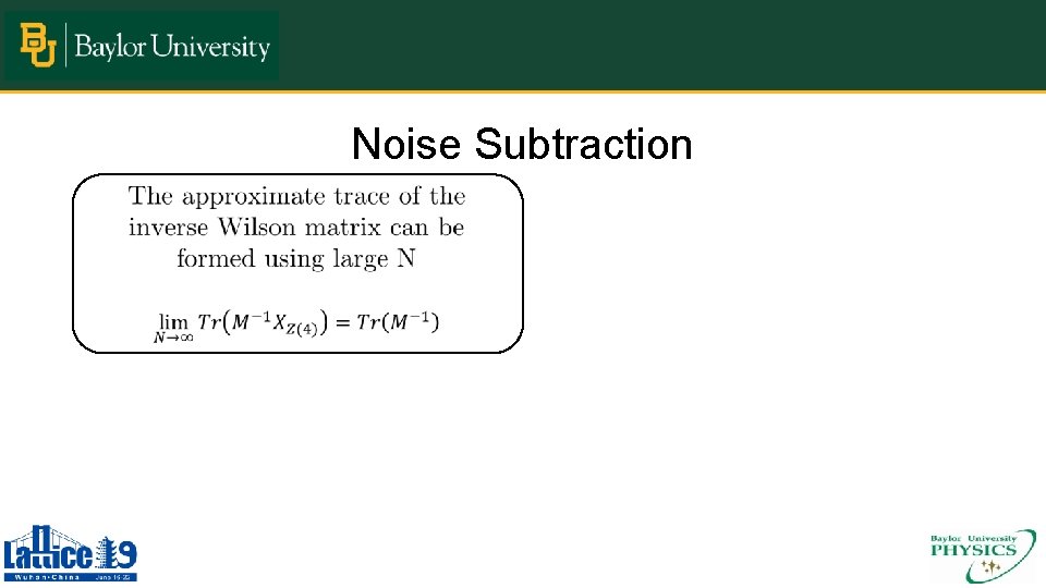
Noise Subtraction
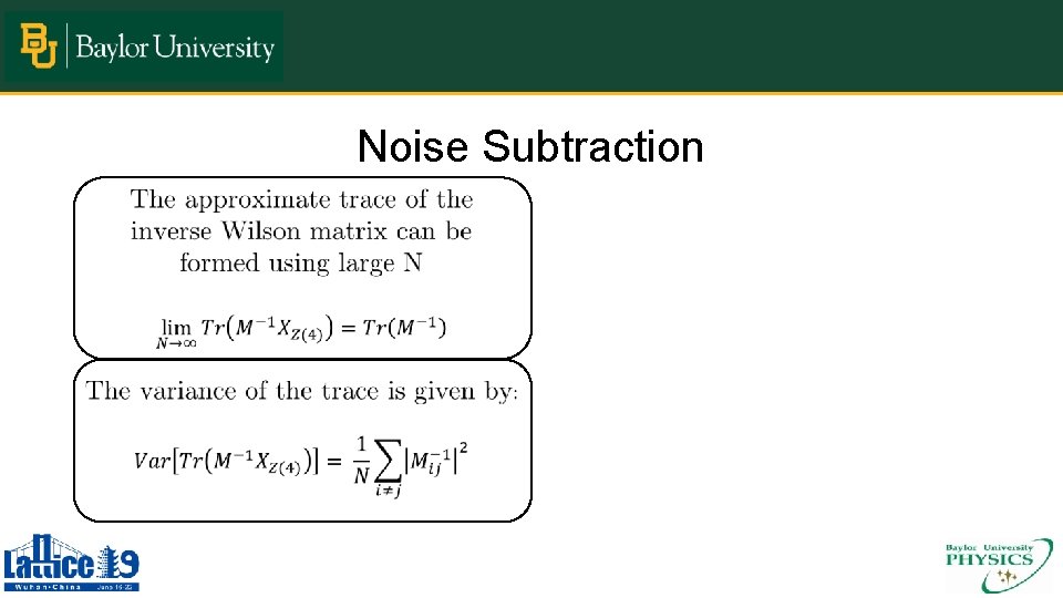
Noise Subtraction
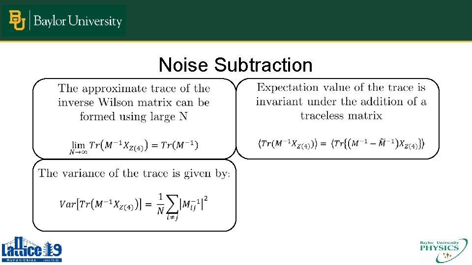
Noise Subtraction
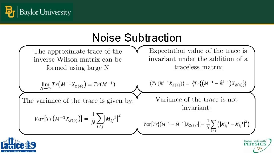
Noise Subtraction
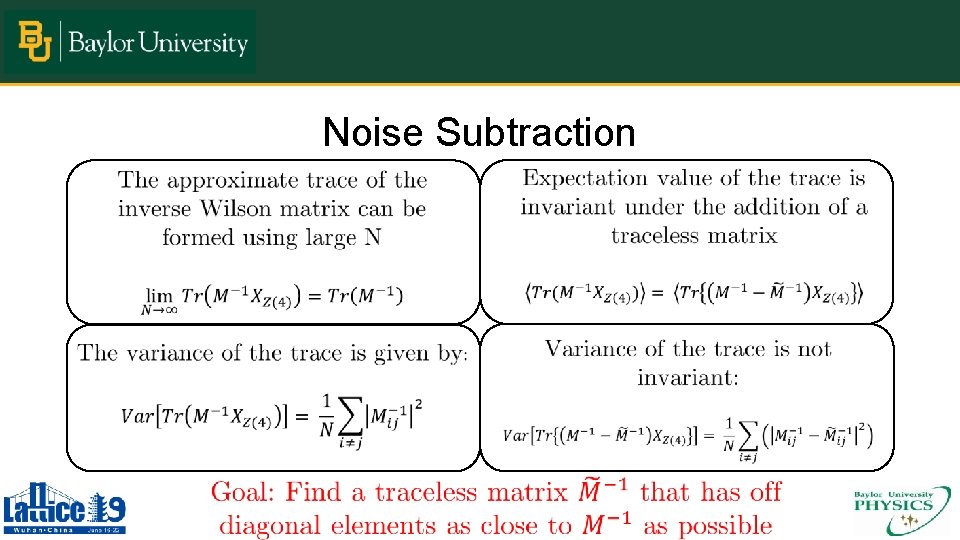
Noise Subtraction

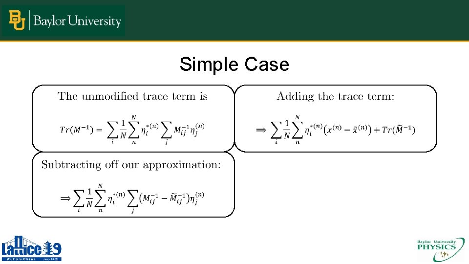
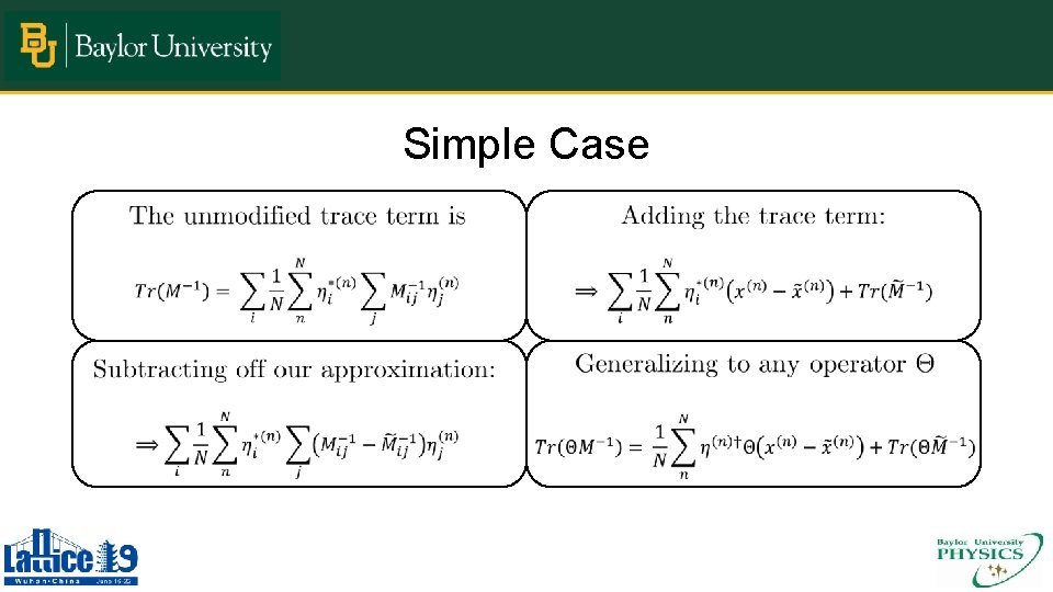
Simple Case
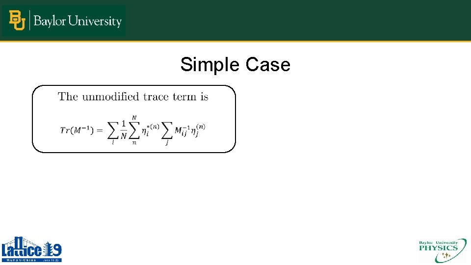
Simple Case
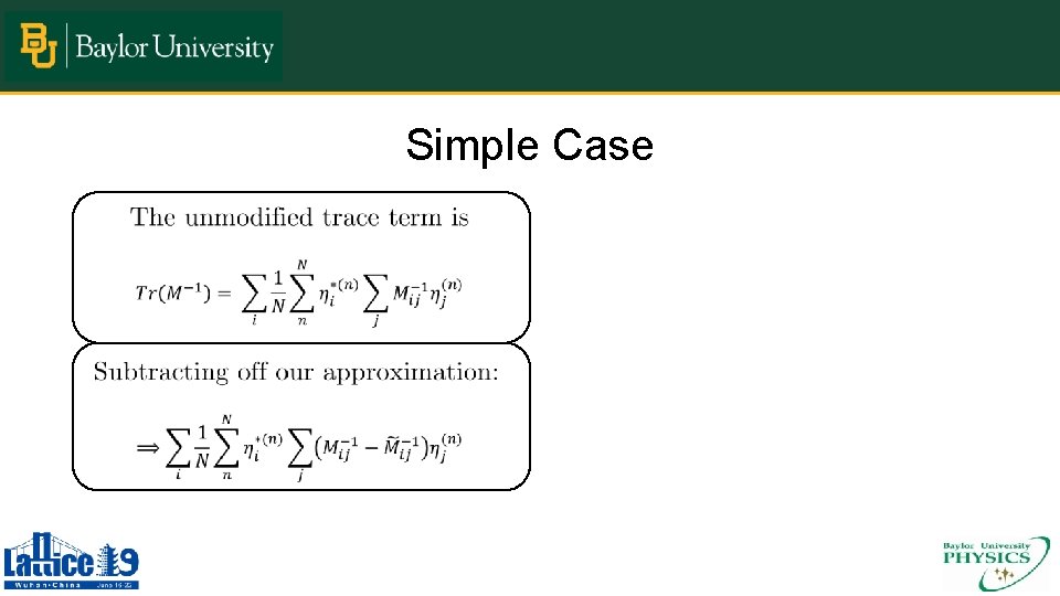
Simple Case
Simple Case
Simple Case

Subtraction Methods

Subtraction Methods Ø No Subtraction (NS)
Subtraction Methods Ø No Subtraction (NS) Ø Eigenvalue Subtraction (ES)
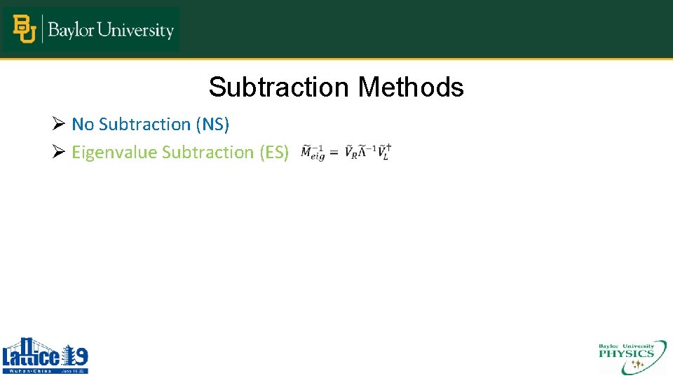
Subtraction Methods Ø No Subtraction (NS) Ø Eigenvalue Subtraction (ES)
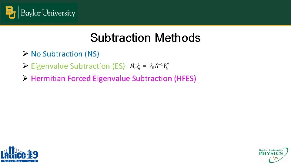
Subtraction Methods Ø No Subtraction (NS) Ø Eigenvalue Subtraction (ES) Ø Hermitian Forced Eigenvalue Subtraction (HFES)
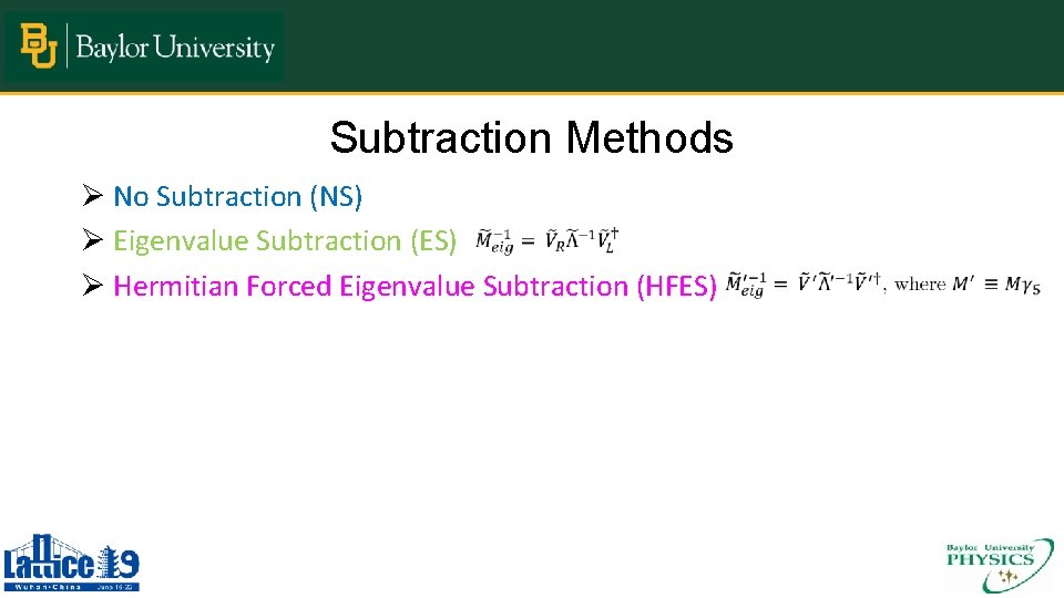
Subtraction Methods Ø No Subtraction (NS) Ø Eigenvalue Subtraction (ES) Ø Hermitian Forced Eigenvalue Subtraction (HFES)
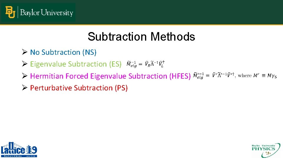
Subtraction Methods Ø No Subtraction (NS) Ø Eigenvalue Subtraction (ES) Ø Hermitian Forced Eigenvalue Subtraction (HFES) Ø Perturbative Subtraction (PS)
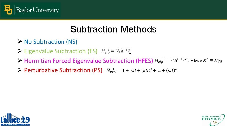
Subtraction Methods Ø No Subtraction (NS) Ø Eigenvalue Subtraction (ES) Ø Hermitian Forced Eigenvalue Subtraction (HFES) Ø Perturbative Subtraction (PS)
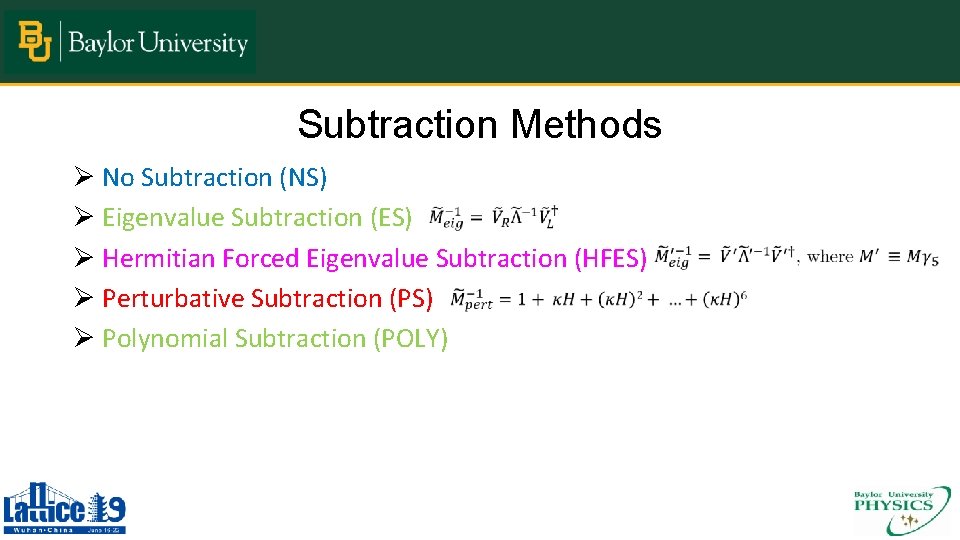
Subtraction Methods Ø No Subtraction (NS) Ø Eigenvalue Subtraction (ES) Ø Hermitian Forced Eigenvalue Subtraction (HFES) Ø Perturbative Subtraction (PS) Ø Polynomial Subtraction (POLY)
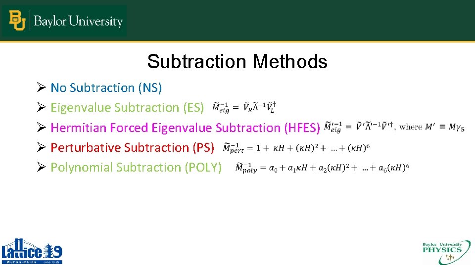
Subtraction Methods Ø No Subtraction (NS) Ø Eigenvalue Subtraction (ES) Ø Hermitian Forced Eigenvalue Subtraction (HFES) Ø Perturbative Subtraction (PS) Ø Polynomial Subtraction (POLY)
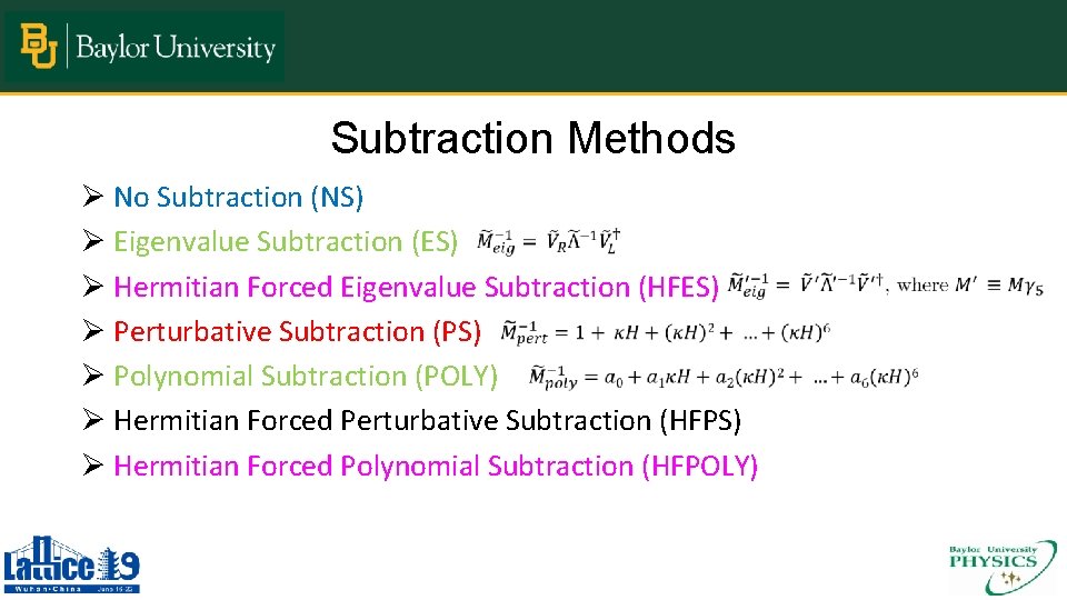
Subtraction Methods Ø No Subtraction (NS) Ø Eigenvalue Subtraction (ES) Ø Hermitian Forced Eigenvalue Subtraction (HFES) Ø Perturbative Subtraction (PS) Ø Polynomial Subtraction (POLY) Ø Hermitian Forced Perturbative Subtraction (HFPS) Ø Hermitian Forced Polynomial Subtraction (HFPOLY)
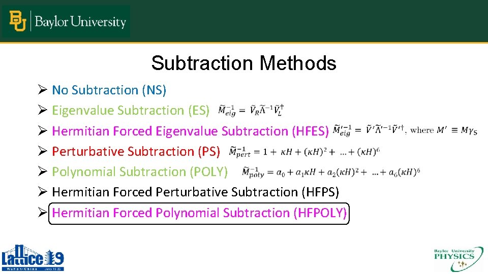
Subtraction Methods Ø No Subtraction (NS) Ø Eigenvalue Subtraction (ES) Ø Hermitian Forced Eigenvalue Subtraction (HFES) Ø Perturbative Subtraction (PS) Ø Polynomial Subtraction (POLY) Ø Hermitian Forced Perturbative Subtraction (HFPS) Ø Hermitian Forced Polynomial Subtraction (HFPOLY)
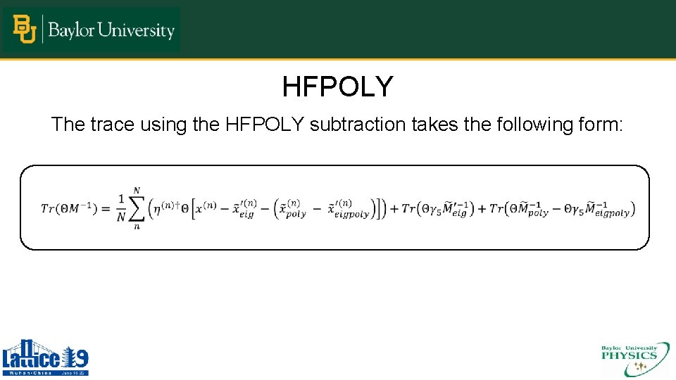
HFPOLY The trace using the HFPOLY subtraction takes the following form:
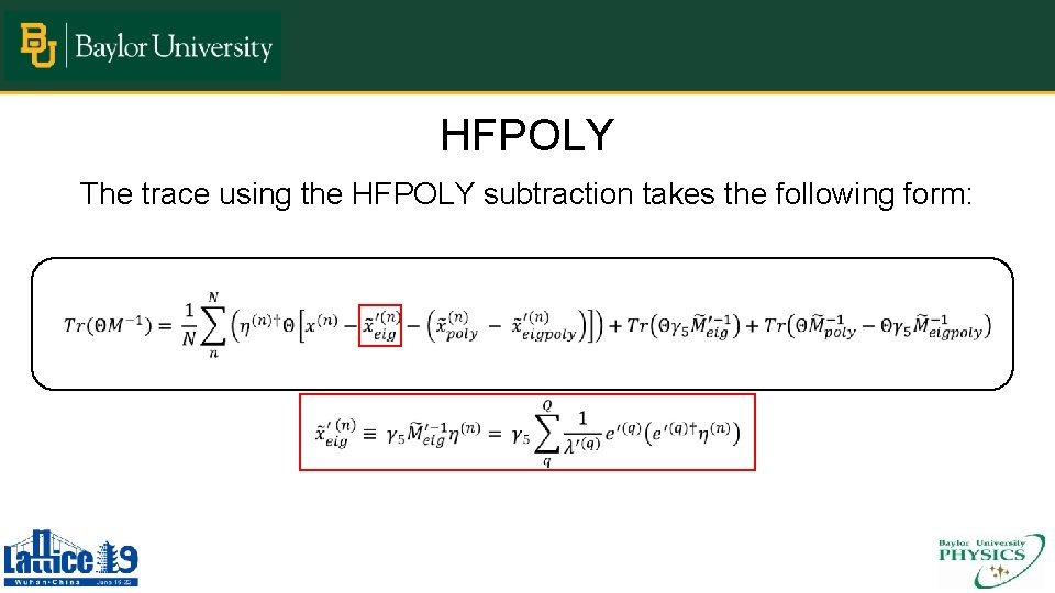
HFPOLY The trace using the HFPOLY subtraction takes the following form:
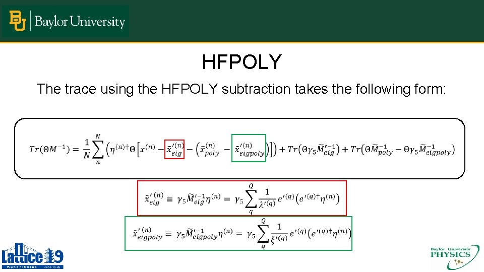
HFPOLY The trace using the HFPOLY subtraction takes the following form:
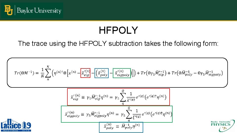
HFPOLY The trace using the HFPOLY subtraction takes the following form:
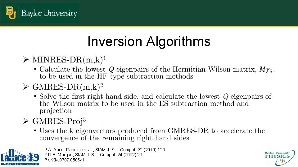
Inversion Algorithms • A. Abdel-Raheim et. al. , SIAM J. Sci. Comput. 32 (2010) 129 R. B. Morgan, SIAM J. Sci. Comput. 24 (2002) 20 3 ar. Xiv: 0707. 0505 v 1 1 2
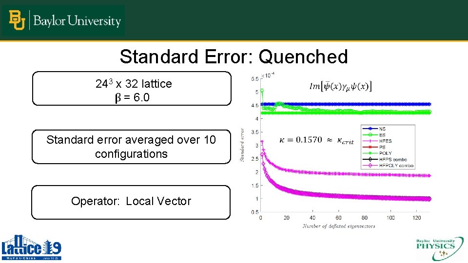
Standard Error: Quenched 243 x 32 lattice β = 6. 0 Standard error averaged over 10 configurations Operator: Local Vector
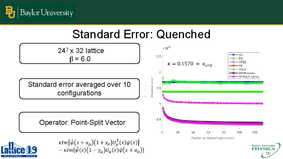
Standard Error: Quenched 243 x 32 lattice β = 6. 0 Standard error averaged over 10 configurations Operator: Point-Split Vector
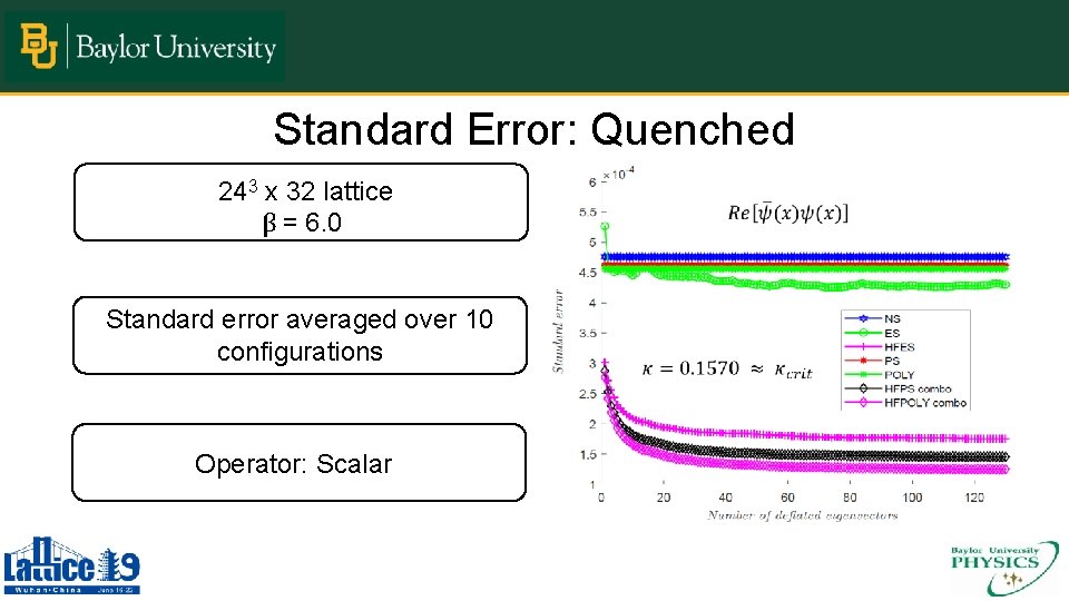
Standard Error: Quenched 243 x 32 lattice β = 6. 0 Standard error averaged over 10 configurations Operator: Scalar
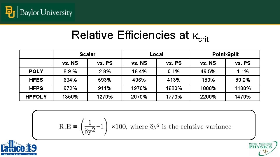
Relative Efficiencies at κcrit Scalar Local Point-Split vs. NS vs. PS POLY 8. 9 % 2. 8% 16. 4% 0. 1% 49. 5% 1. 1% HFES 634% 593% 496% 413% 180% 89. 2% HFPS 972% 911% 1970% 1680% 1800% 1180% HFPOLY 1350% 1270% 2070% 1770% 2200% 1470%
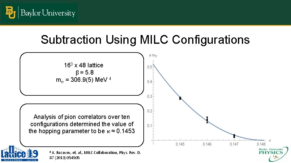
Subtraction Using MILC Configurations 163 x 48 lattice β = 5. 8 mπ = 306. 9(5) Me. V 4 Analysis of pion correlators over ten configurations determined the value of the hopping parameter to be κ ≈ 0. 1453 4 A. Bazavov, et. al. , MILC Collaboration, Phys. Rev. D. 87 (2013) 054505
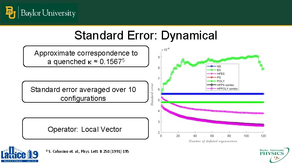
Standard Error: Dynamical Approximate correspondence to a quenched κ ≈ 0. 15675 Standard error averaged over 10 configurations Operator: Local Vector 5 S. Cabasino et. al. , Phys. Lett. B 258 (1991) 195
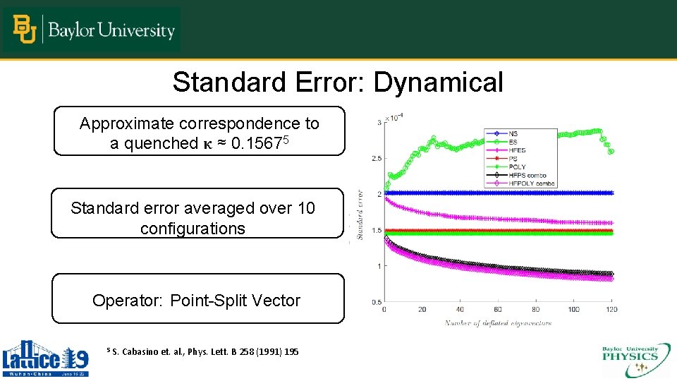
Standard Error: Dynamical Approximate correspondence to a quenched κ ≈ 0. 15675 Standard error averaged over 10 configurations Operator: Point-Split Vector 5 S. Cabasino et. al. , Phys. Lett. B 258 (1991) 195
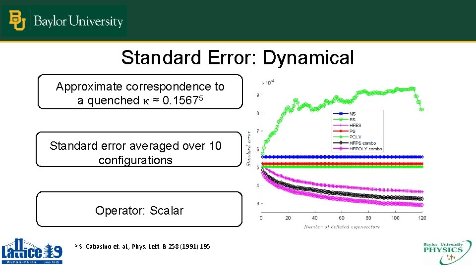
Standard Error: Dynamical Approximate correspondence to a quenched κ ≈ 0. 15675 Standard error averaged over 10 configurations Operator: Scalar 5 S. Cabasino et. al. , Phys. Lett. B 258 (1991) 195
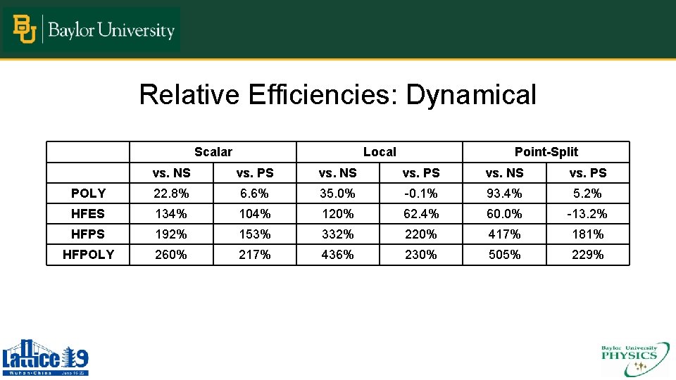
Relative Efficiencies: Dynamical Scalar Local Point-Split vs. NS vs. PS POLY 22. 8% 6. 6% 35. 0% -0. 1% 93. 4% 5. 2% HFES 134% 104% 120% 62. 4% 60. 0% -13. 2% HFPS 192% 153% 332% 220% 417% 181% HFPOLY 260% 217% 436% 230% 505% 229%
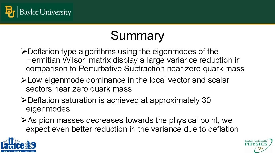
Summary ØDeflation type algorithms using the eigenmodes of the Hermitian Wilson matrix display a large variance reduction in comparison to Perturbative Subtraction near zero quark mass ØLow eigenmode dominance in the local vector and scalar sectors near zero quark mass ØDeflation saturation is achieved at approximately 30 eigenmodes ØAs pion masses decreases towards the physical point, we expect even better reduction in the variance due to deflation

Acknowledgments Thank you to the Organizing Committee of Lattice 2019 for providing accommodations, Doug Toussaint, Carlton De. Tar, Jim Hetrick for their help in obtaining the MILC configurations, and Abdou Abdel-Raheim, Victor Guerrero and Paul Lashomb for their help in this study. This work was partially supported through the Baylor University Research Committee and the Texas Advanced Super Computing Center
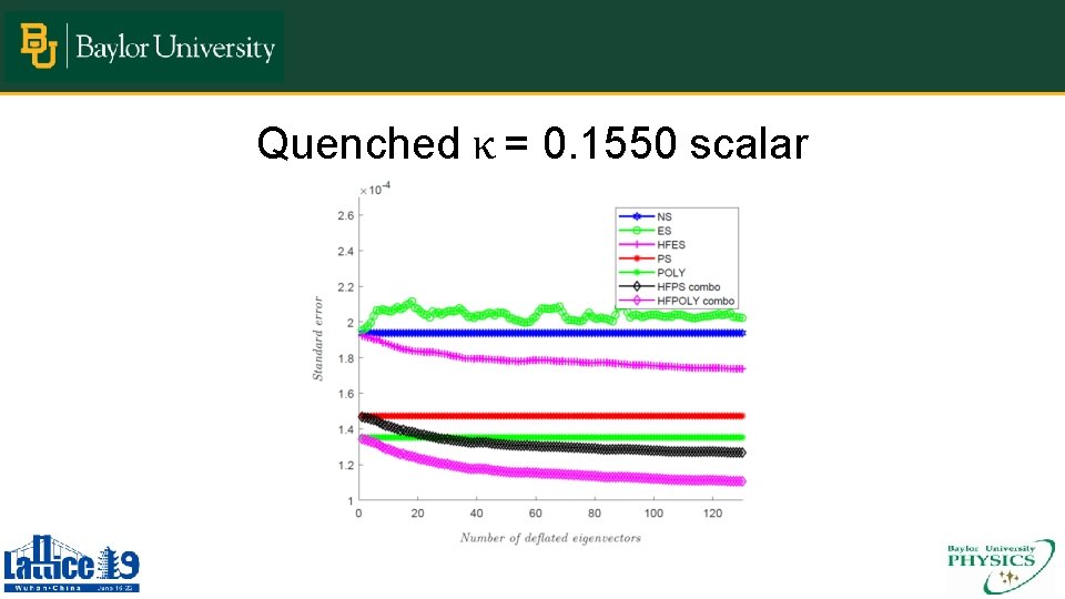
Quenched κ = 0. 1550 scalar
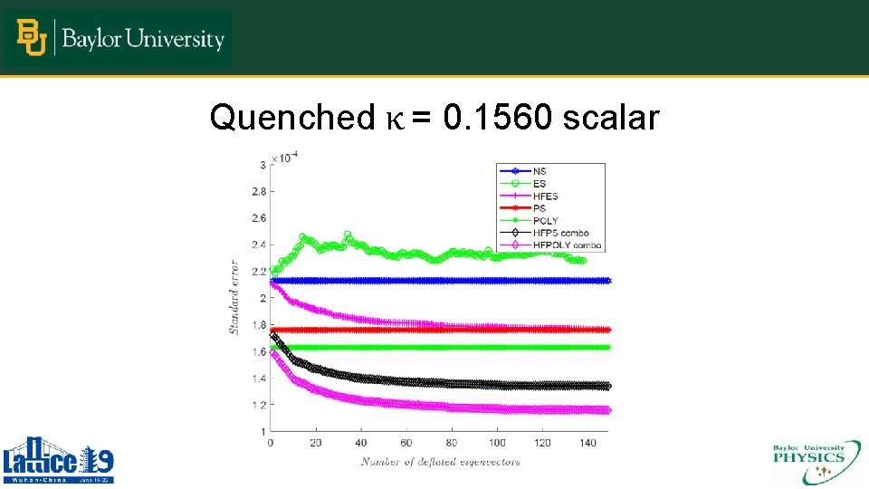
Quenched κ = 0. 1560 scalar
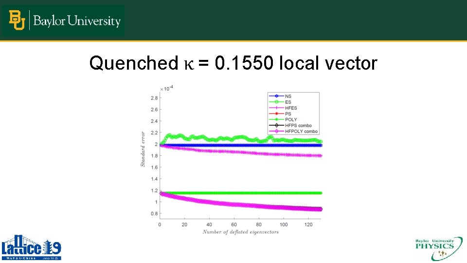
Quenched κ = 0. 1550 local vector
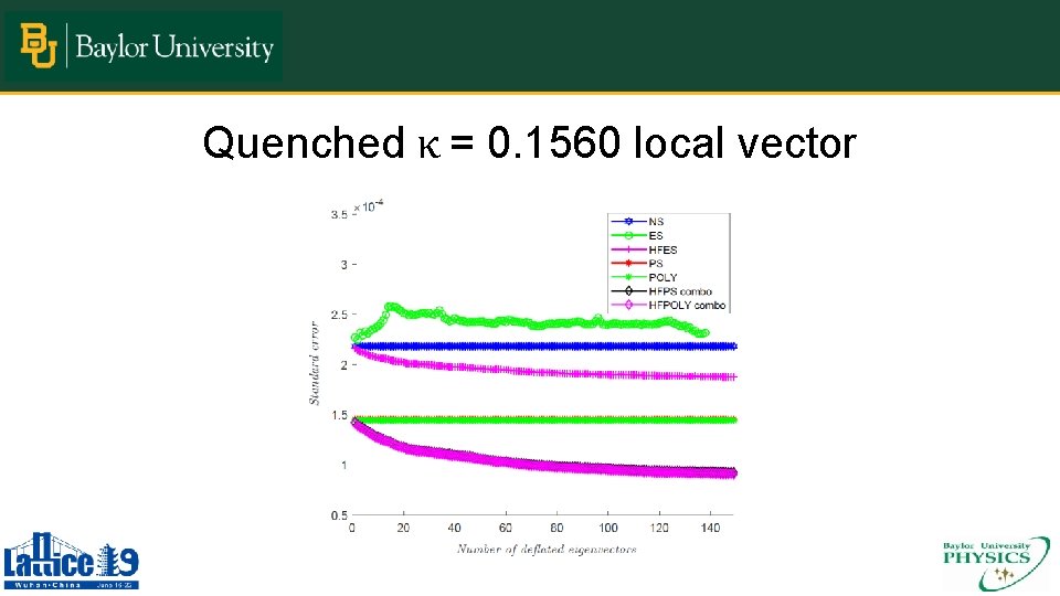
Quenched κ = 0. 1560 local vector
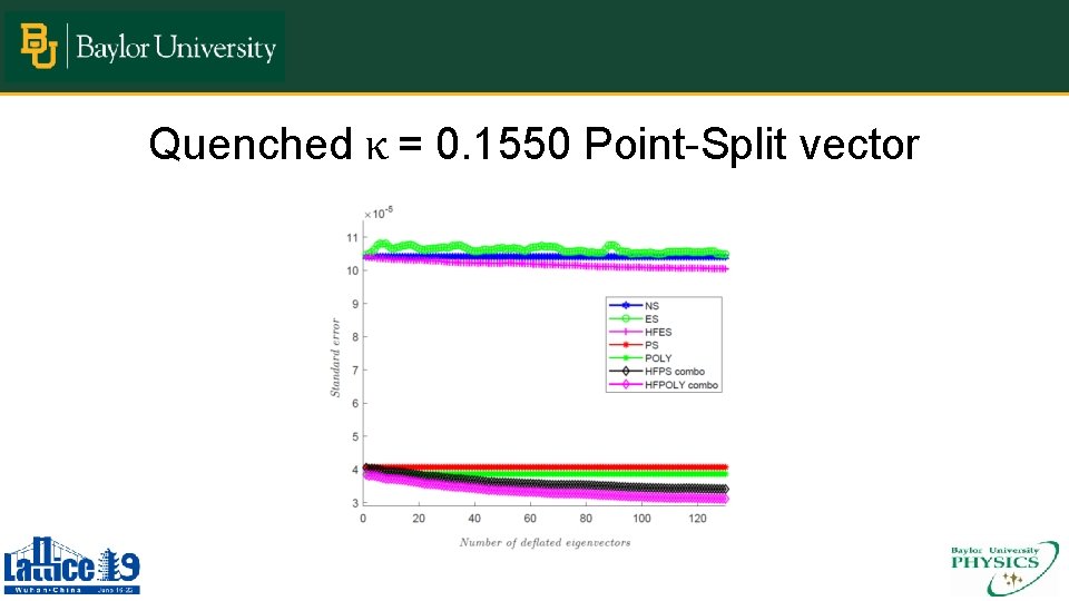
Quenched κ = 0. 1550 Point-Split vector
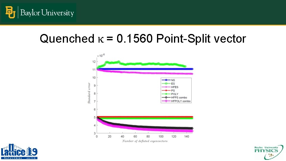
Quenched κ = 0. 1560 Point-Split vector
- Slides: 53