Disciplined Software Engineering Lecture 4 Software Engineering Institute

- Slides: 42

Disciplined Software Engineering Lecture #4 Software Engineering Institute Carnegie Mellon University Pittsburgh, PA 15213 Sponsored by the U. S. Department of Defense Copyright © 1994 Carnegie Mellon University Disciplined Software Engineering - Lecture 1 1

Lecture #4 Overview - Estimating Software Size - 2 Size estimating overview The PROBE estimating method Categorizing object data The regression method Process additions Copyright © 1994 Carnegie Mellon University Disciplined Software Engineering - Lecture 1 2

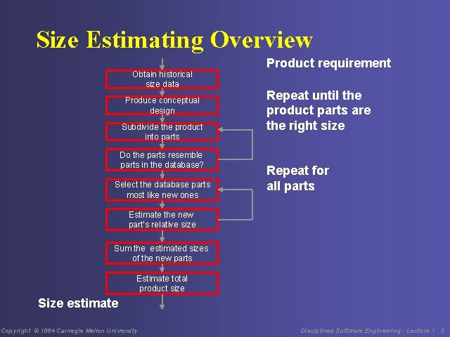
Size Estimating Overview Obtain historical size data Produce conceptual design Subdivide the product into parts Do the parts resemble parts in the database? Select the database parts most like new ones Product requirement Repeat until the product parts are the right size Repeat for all parts Estimate the new part’s relative size Sum the estimated sizes of the new parts Estimate total product size Size estimate Copyright © 1994 Carnegie Mellon University Disciplined Software Engineering - Lecture 1 3

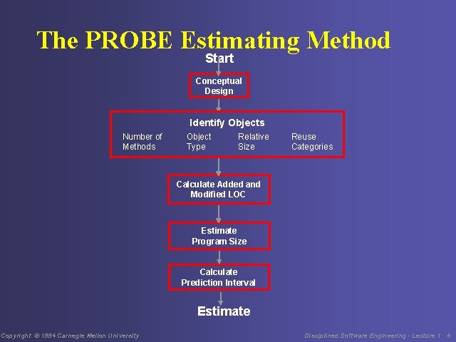
The PROBE Estimating Method Start Conceptual Design Identify Objects Number of Methods Object Type Relative Size Reuse Categories Calculate Added and Modified LOC Estimate Program Size Calculate Prediction Interval Estimate Copyright © 1994 Carnegie Mellon University Disciplined Software Engineering - Lecture 1 4

PROBE Method Description The following charts describe the PROBE method. Use form C 39 in Appendix C (page 683) as a reference during the discussion. The examples are taken from Table 5. 8 in Chapter 5 (page 120). Copyright © 1994 Carnegie Mellon University Disciplined Software Engineering - Lecture 1 5

Conceptual Design A conceptual design is needed • to relate the requirements to the product • to define the product elements that will produce the desired functions • to estimate the size of what will be built For understood designs, conceptual designs can be done quickly. If you do not understand the design, you do not know enough to make an estimate. Copyright © 1994 Carnegie Mellon University Disciplined Software Engineering - Lecture 1 6

Identify the Objects - 1 Where possible, select application entities. Judge how many methods each object will likely contain. Determine the type of the object, i. e. : data, calculation, file, control, etc. Judge the relative size of each object: very small (VS), small (S), medium (M), large (L), very large (VL). Copyright © 1994 Carnegie Mellon University Disciplined Software Engineering - Lecture 1 7

Identify the Objects - 2 From historical object data, determine the size in LOC/method of each object. Multiply by the number of methods to get the estimated object LOC. Judge which objects will be added to the reuse library and note as “New Reused. ” Copyright © 1994 Carnegie Mellon University Disciplined Software Engineering - Lecture 1 8

Identify the Objects - 3 When objects do not fit an existing type, they are frequently composites. • Ensure they are sufficiently refined • Refine those that are not elemental objects Watch for new object types Copyright © 1994 Carnegie Mellon University Disciplined Software Engineering - Lecture 1 9

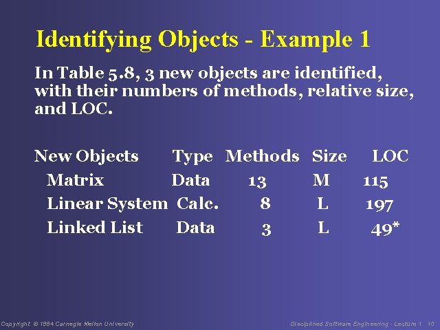
Identifying Objects - Example 1 In Table 5. 8, 3 new objects are identified, with their numbers of methods, relative size, and LOC. New Objects Type Methods Size LOC Matrix Data 13 M 115 Linear System Calc. 8 L 197 Linked List Data 3 L 49* Copyright © 1994 Carnegie Mellon University Disciplined Software Engineering - Lecture 1 10

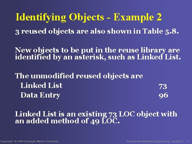
Identifying Objects - Example 2 3 reused objects are also shown in Table 5. 8. New objects to be put in the reuse library are identified by an asterisk, such as Linked List. The unmodified reused objects are Linked List Data Entry 73 96 Linked List is an existing 73 LOC object with an added method of 49 LOC. Copyright © 1994 Carnegie Mellon University Disciplined Software Engineering - Lecture 1 11

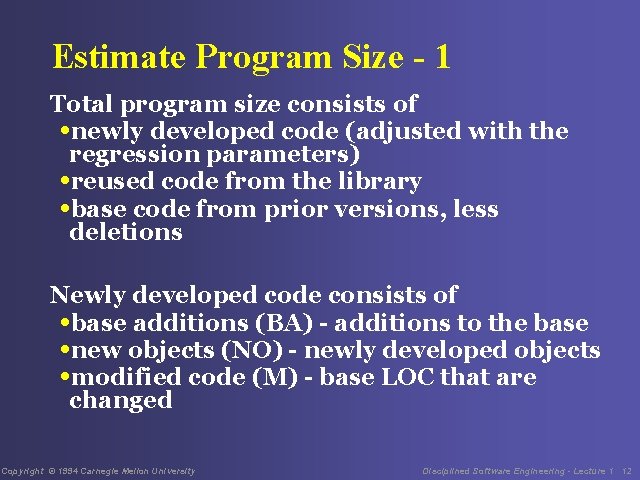
Estimate Program Size - 1 Total program size consists of • newly developed code (adjusted with the regression parameters) • reused code from the library • base code from prior versions, less deletions Newly developed code consists of • base additions (BA) - additions to the base • new objects (NO) - newly developed objects • modified code (M) - base LOC that are changed Copyright © 1994 Carnegie Mellon University Disciplined Software Engineering - Lecture 1 12

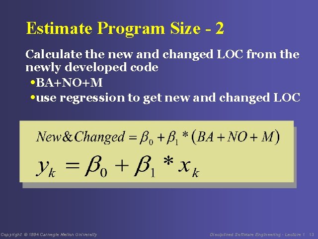
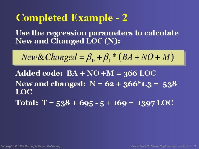
Estimate Program Size - 2 Calculate the new and changed LOC from the newly developed code • BA+NO+M • use regression to get new and changed LOC Copyright © 1994 Carnegie Mellon University Disciplined Software Engineering - Lecture 1 13

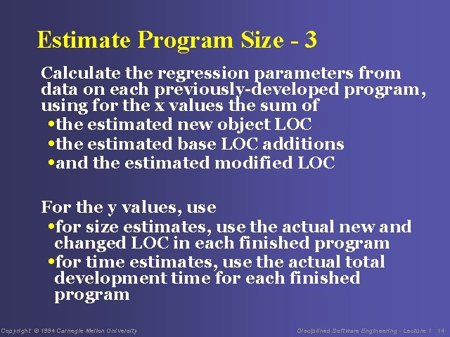
Estimate Program Size - 3 Calculate the regression parameters from data on each previously-developed program, using for the x values the sum of • the estimated new object LOC • the estimated base LOC additions • and the estimated modified LOC For the y values, use • for size estimates, use the actual new and changed LOC in each finished program • for time estimates, use the actual total development time for each finished program Copyright © 1994 Carnegie Mellon University Disciplined Software Engineering - Lecture 1 14

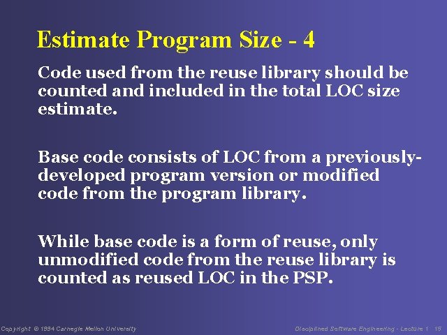
Estimate Program Size - 4 Code used from the reuse library should be counted and included in the total LOC size estimate. Base code consists of LOC from a previouslydeveloped program version or modified code from the program library. While base code is a form of reuse, only unmodified code from the reuse library is counted as reused LOC in the PSP. Copyright © 1994 Carnegie Mellon University Disciplined Software Engineering - Lecture 1 15

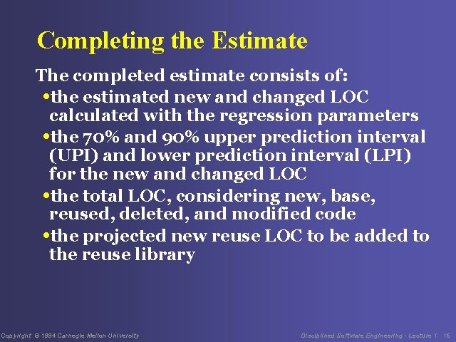
Completing the Estimate The completed estimate consists of: • the estimated new and changed LOC calculated with the regression parameters • the 70% and 90% upper prediction interval (UPI) and lower prediction interval (LPI) for the new and changed LOC • the total LOC, considering new, base, reused, deleted, and modified code • the projected new reuse LOC to be added to the reuse library Copyright © 1994 Carnegie Mellon University Disciplined Software Engineering - Lecture 1 16

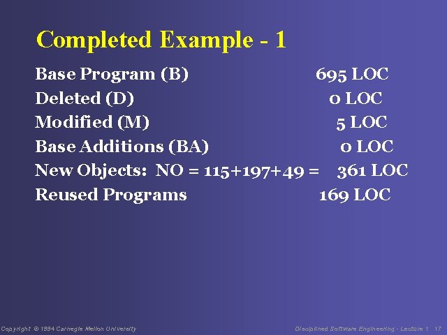
Completed Example - 1 Base Program (B) 695 LOC Deleted (D) 0 LOC Modified (M) 5 LOC Base Additions (BA) 0 LOC New Objects: NO = 115+197+49 = 361 LOC Reused Programs 169 LOC Copyright © 1994 Carnegie Mellon University Disciplined Software Engineering - Lecture 1 17

Completed Example - 2 Use the regression parameters to calculate New and Changed LOC (N): Added code: BA + NO +M = 366 LOC New and changed: N = 62 + 366*1. 3 = 538 LOC Total: T = 538 + 695 - 5 + 169 = 1397 LOC Copyright © 1994 Carnegie Mellon University Disciplined Software Engineering - Lecture 1 18

To Make Size Estimates, You Need Several Items Data on historical objects, divided into types Estimating factors for the relative sizes of each object type Regression parameters for computing new and changed LOC from: • estimated object LOC • LOC added to the base • modified LOC Copyright © 1994 Carnegie Mellon University Disciplined Software Engineering - Lecture 1 19

Historical Data on Objects Object size is highly variable • depends on language • influenced by design style • helps to normalize by number of methods Pick basic types • logic, control • I/O, files, display • data, text, calculation • set-up, error handling Copyright © 1994 Carnegie Mellon University Disciplined Software Engineering - Lecture 1 20

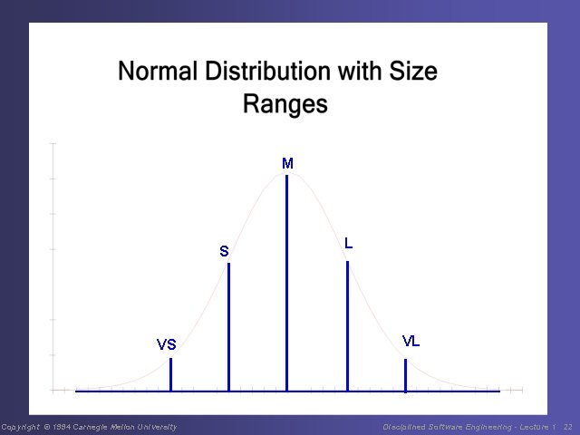
Estimating Factors for Objects You seek size ranges for each type that will help you judge the sizes of new objects. To calculate these size ranges • take the mean • take the standard deviation • very small: VS = mean - 2*standard deviations • small: S = mean - standard deviation • medium: M = mean • large: L = mean + standard deviation • very large: VL = mean + 2*standard deviations Copyright © 1994 Carnegie Mellon University Disciplined Software Engineering - Lecture 1 21

M S VS Copyright © 1994 Carnegie Mellon University L VL Disciplined Software Engineering - Lecture 1 22

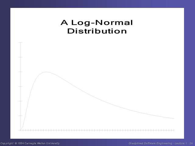
Log-Normal Distribution These size ranges assume the object data are normally distributed. If the data are log-normally distributed, take the log of the data before making the size range calculations. Then, after computing the size ranges, take the antilog to get the factors in LOC Copyright © 1994 Carnegie Mellon University Disciplined Software Engineering - Lecture 1 23

Copyright © 1994 Carnegie Mellon University Disciplined Software Engineering - Lecture 1 24

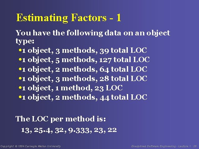
Estimating Factors - 1 You have the following data on an object type: • 1 object, 3 methods, 39 total LOC • 1 object, 5 methods, 127 total LOC • 1 object, 2 methods, 64 total LOC • 1 object, 3 methods, 28 total LOC • 1 object, 1 method, 23 LOC • 1 object, 2 methods, 44 total LOC The LOC per method is: 13, 25. 4, 32, 9. 333, 22 Copyright © 1994 Carnegie Mellon University Disciplined Software Engineering - Lecture 1 25

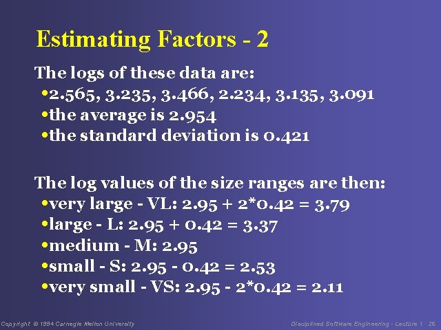
Estimating Factors - 2 The logs of these data are: • 2. 565, 3. 235, 3. 466, 2. 234, 3. 135, 3. 091 • the average is 2. 954 • the standard deviation is 0. 421 The log values of the size ranges are then: • very large - VL: 2. 95 + 2*0. 42 = 3. 79 • large - L: 2. 95 + 0. 42 = 3. 37 • medium - M: 2. 95 • small - S: 2. 95 - 0. 42 = 2. 53 • very small - VS: 2. 95 - 2*0. 42 = 2. 11 Copyright © 1994 Carnegie Mellon University Disciplined Software Engineering - Lecture 1 26

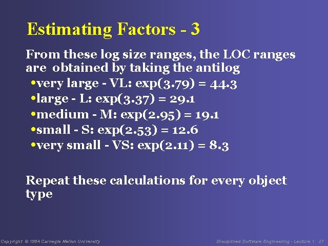
Estimating Factors - 3 From these log size ranges, the LOC ranges are obtained by taking the antilog • very large - VL: exp(3. 79) = 44. 3 • large - L: exp(3. 37) = 29. 1 • medium - M: exp(2. 95) = 19. 1 • small - S: exp(2. 53) = 12. 6 • very small - VS: exp(2. 11) = 8. 3 Repeat these calculations for every object type Copyright © 1994 Carnegie Mellon University Disciplined Software Engineering - Lecture 1 27

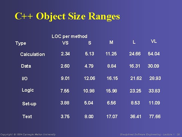
C++ Object Size Ranges Type LOC per method VS S M L VL Calculation 2. 34 5. 13 11. 25 24. 66 54. 04 Data 2. 60 4. 79 8. 84 16. 31 30. 09 I/O 9. 01 12. 06 16. 15 21. 62 28. 93 Logic 7. 55 10. 98 15. 98 23. 25 33. 83 Set-up 3. 88 5. 04 6. 56 8. 53 11. 09 Text 3. 75 8. 00 17. 07 36. 41 77. 66 Copyright © 1994 Carnegie Mellon University Disciplined Software Engineering - Lecture 1 28

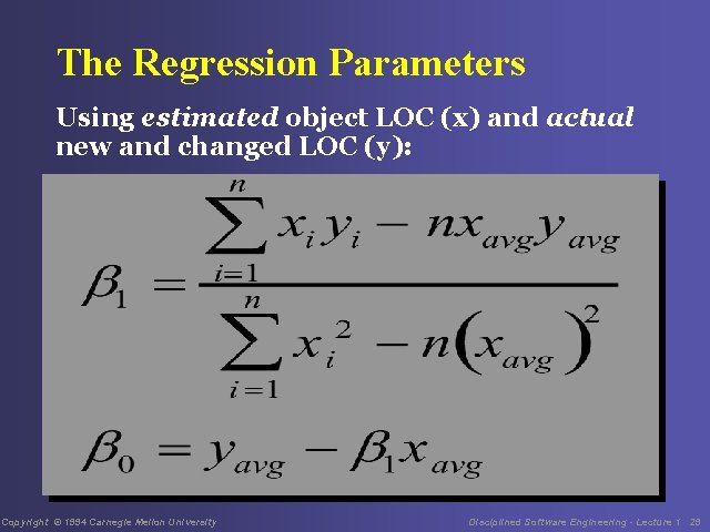
The Regression Parameters Using estimated object LOC (x) and actual new and changed LOC (y): Copyright © 1994 Carnegie Mellon University Disciplined Software Engineering - Lecture 1 29

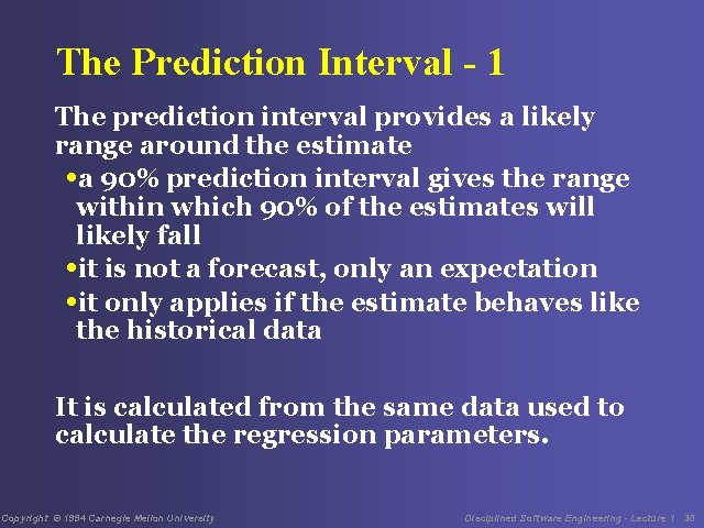
The Prediction Interval - 1 The prediction interval provides a likely range around the estimate • a 90% prediction interval gives the range within which 90% of the estimates will likely fall • it is not a forecast, only an expectation • it only applies if the estimate behaves like the historical data It is calculated from the same data used to calculate the regression parameters. Copyright © 1994 Carnegie Mellon University Disciplined Software Engineering - Lecture 1 30

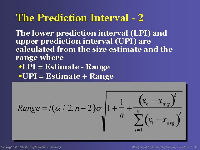
The Prediction Interval - 2 The lower prediction interval (LPI) and upper prediction interval (UPI) are calculated from the size estimate and the range where • LPI = Estimate - Range • UPI = Estimate + Range Copyright © 1994 Carnegie Mellon University Disciplined Software Engineering - Lecture 1 31

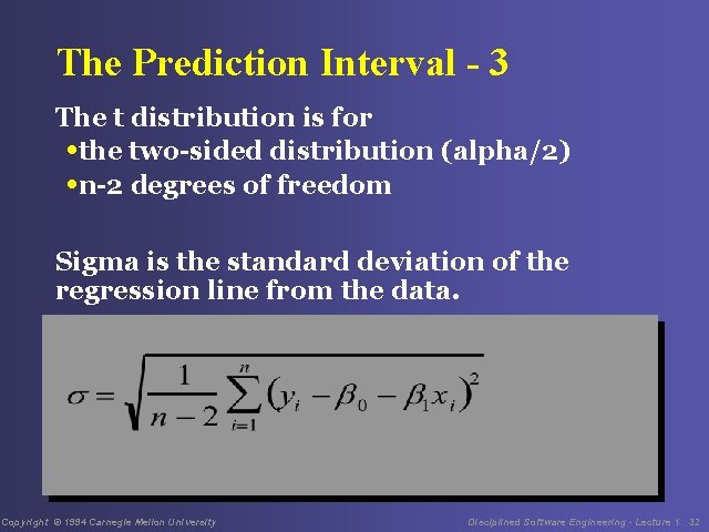
The Prediction Interval - 3 The t distribution is for • the two-sided distribution (alpha/2) • n-2 degrees of freedom Sigma is the standard deviation of the regression line from the data. Copyright © 1994 Carnegie Mellon University Disciplined Software Engineering - Lecture 1 32

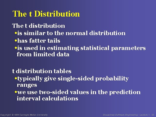
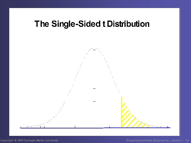
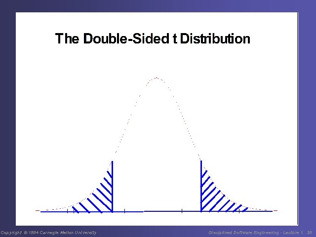
The t Distribution The t distribution • is similar to the normal distribution • has fatter tails • is used in estimating statistical parameters from limited data t distribution tables • typically give single-sided probability ranges • we use two-sided values in the prediction interval calculations Copyright © 1994 Carnegie Mellon University Disciplined Software Engineering - Lecture 1 33

Copyright © 1994 Carnegie Mellon University Disciplined Software Engineering - Lecture 1 34

Copyright © 1994 Carnegie Mellon University Disciplined Software Engineering - Lecture 1 35

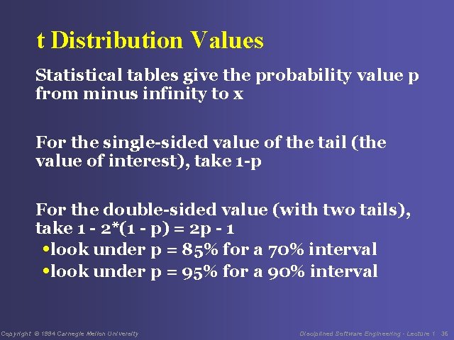
t Distribution Values Statistical tables give the probability value p from minus infinity to x For the single-sided value of the tail (the value of interest), take 1 -p For the double-sided value (with two tails), take 1 - 2*(1 - p) = 2 p - 1 • look under p = 85% for a 70% interval • look under p = 95% for a 90% interval Copyright © 1994 Carnegie Mellon University Disciplined Software Engineering - Lecture 1 36

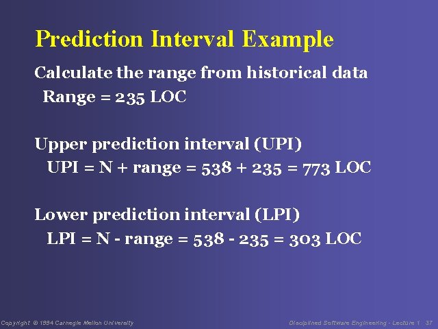
Prediction Interval Example Calculate the range from historical data Range = 235 LOC Upper prediction interval (UPI) UPI = N + range = 538 + 235 = 773 LOC Lower prediction interval (LPI) LPI = N - range = 538 - 235 = 303 LOC Copyright © 1994 Carnegie Mellon University Disciplined Software Engineering - Lecture 1 37

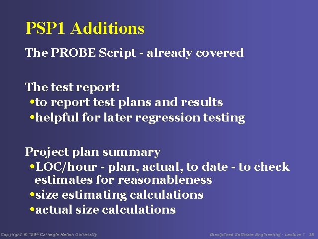
PSP 1 Additions The PROBE Script - already covered The test report: • to report test plans and results • helpful for later regression testing Project plan summary • LOC/hour - plan, actual, to date - to check estimates for reasonableness • size estimating calculations • actual size calculations Copyright © 1994 Carnegie Mellon University Disciplined Software Engineering - Lecture 1 38

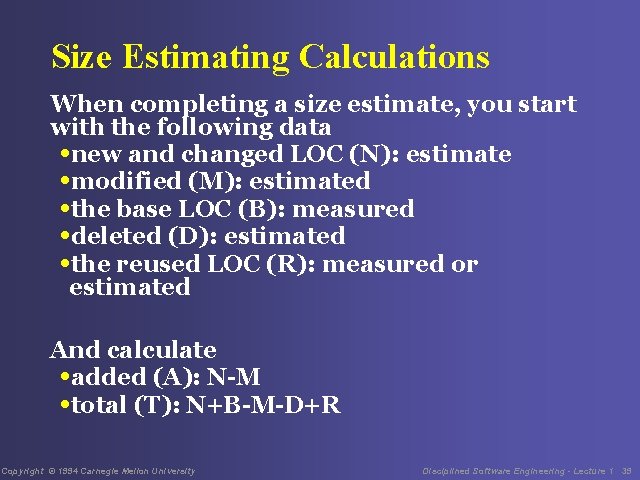
Size Estimating Calculations When completing a size estimate, you start with the following data • new and changed LOC (N): estimate • modified (M): estimated • the base LOC (B): measured • deleted (D): estimated • the reused LOC (R): measured or estimated And calculate • added (A): N-M • total (T): N+B-M-D+R Copyright © 1994 Carnegie Mellon University Disciplined Software Engineering - Lecture 1 39

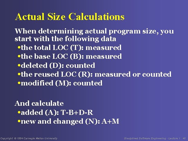
Actual Size Calculations When determining actual program size, you start with the following data • the total LOC (T): measured • the base LOC (B): measured • deleted (D): counted • the reused LOC (R): measured or counted • modified (M): counted And calculate • added (A): T-B+D-R • new and changed (N): A+M Copyright © 1994 Carnegie Mellon University Disciplined Software Engineering - Lecture 1 40

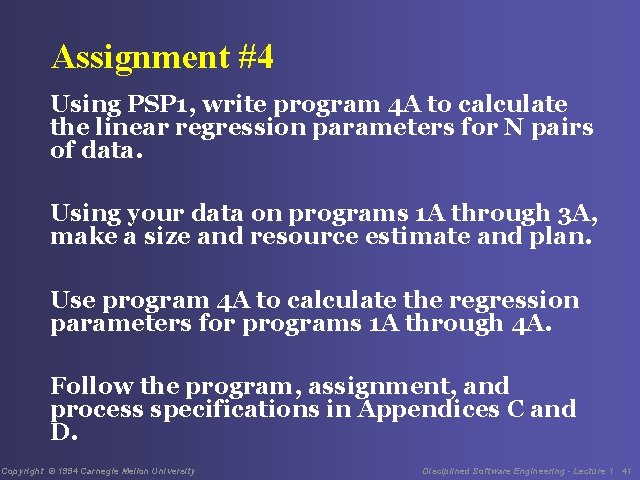
Assignment #4 Using PSP 1, write program 4 A to calculate the linear regression parameters for N pairs of data. Using your data on programs 1 A through 3 A, make a size and resource estimate and plan. Use program 4 A to calculate the regression parameters for programs 1 A through 4 A. Follow the program, assignment, and process specifications in Appendices C and D. Copyright © 1994 Carnegie Mellon University Disciplined Software Engineering - Lecture 1 41

Messages to Remember from Lecture 4 1 - The PROBE method is a structured way to make software size estimates. 2 - It uses your personal size data. 3 - It provides a statistically sound range within which the actual program size will most likely fall. Copyright © 1994 Carnegie Mellon University Disciplined Software Engineering - Lecture 1 42