Directed Acyclic Graphs An Application to Modeling Causal

Directed Acyclic Graphs: An Application to Modeling Causal Relationships with Worldwide Poverty Data Gott würfelt nicht. -- Albert Einstein David A. Bessler Texas A&M University Presented to James S. Mc. Donnell Foundation 21 st Century Science Initiative “Creating Knowledge from Information” Tarrytown, New York June 3, 2003 1

Outline u Poverty literature u Causal modeling and directed graphs u Directed graphs on poverty variables u Regression, front door, and back door paths u Summary and caution 2

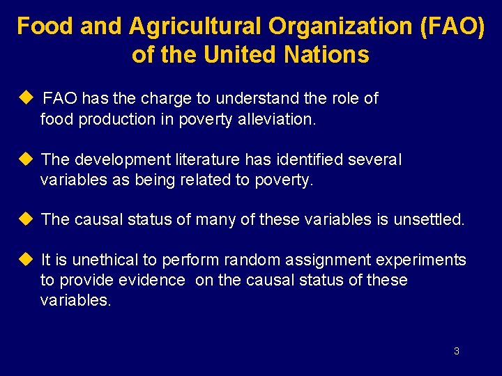
Food and Agricultural Organization (FAO) of the United Nations u FAO has the charge to understand the role of food production in poverty alleviation. u The development literature has identified several variables as being related to poverty. u The causal status of many of these variables is unsettled. u It is unethical to perform random assignment experiments to provide evidence on the causal status of these variables. 3

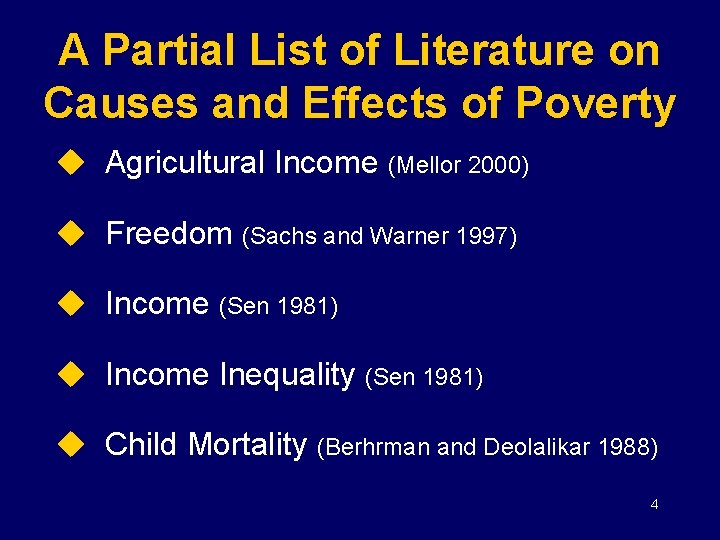
A Partial List of Literature on Causes and Effects of Poverty u Agricultural Income (Mellor 2000) u Freedom (Sachs and Warner 1997) u Income (Sen 1981) u Income Inequality (Sen 1981) u Child Mortality (Berhrman and Deolalikar 1988) 4

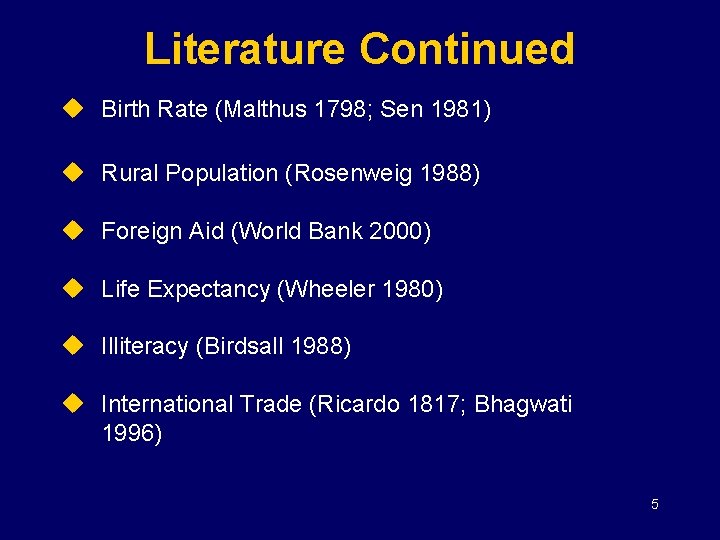
Literature Continued u Birth Rate (Malthus 1798; Sen 1981) u Rural Population (Rosenweig 1988) u Foreign Aid (World Bank 2000) u Life Expectancy (Wheeler 1980) u Illiteracy (Birdsall 1988) u International Trade (Ricardo 1817; Bhagwati 1996) 5

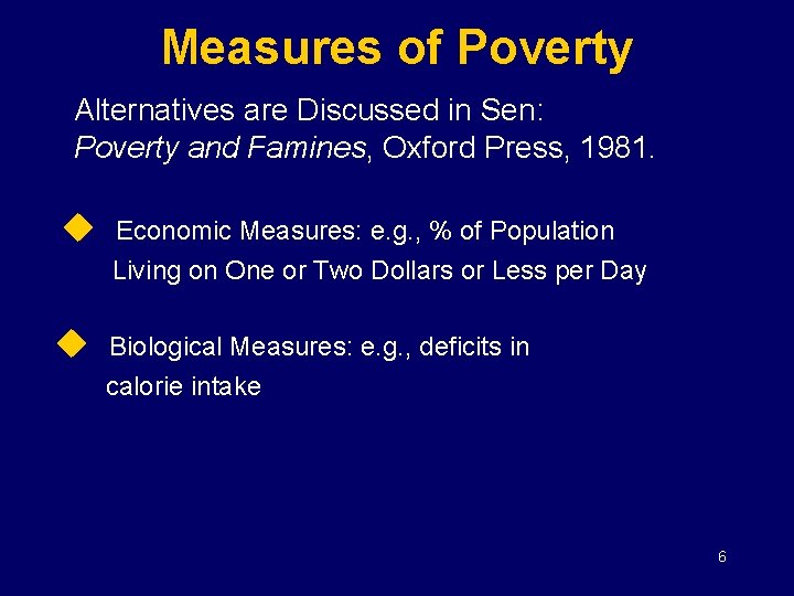
Measures of Poverty Alternatives are Discussed in Sen: Poverty and Famines, Oxford Press, 1981. u Economic Measures: e. g. , % of Population Living on One or Two Dollars or Less per Day u Biological Measures: e. g. , deficits in calorie intake 6

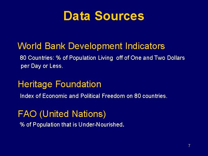
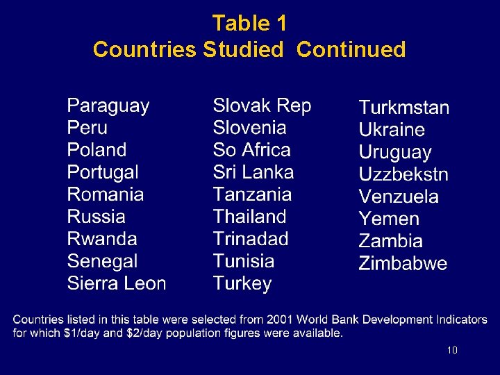
Data Sources World Bank Development Indicators 80 Countries: % of Population Living off of One and Two Dollars per Day or Less. Heritage Foundation Index of Economic and Political Freedom on 80 countries. FAO (United Nations) % of Population that is Under-Nourished. 7

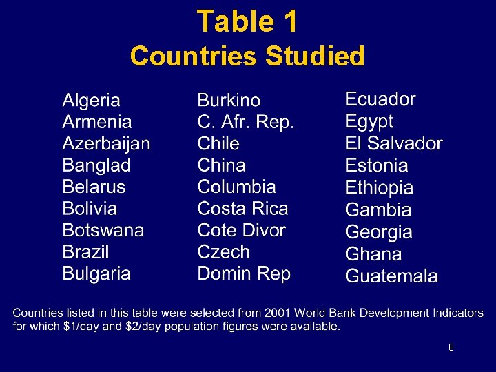
Table 1 Countries Studied 8

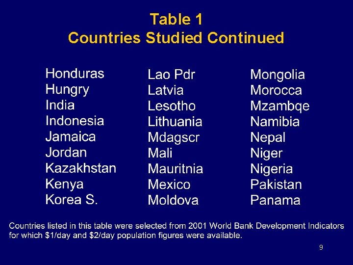
Table 1 Countries Studied Continued 9

Table 1 Countries Studied Continued 10

Inference on Causal Flows u Oftentimes we are uncertain about which variables are causal in a modeling effort. u Theory may tell us what our fundamental causal variables are in a controlled system. u It is common that our data may not be collected in a controlled environment. 11

Use of Subject Matter Theory may be a good source of information about direction of causal flow among variables. However, theory usually invokes the ceteris paribus condition to achieve results. Data are often observational (non-experimental) and thus the ceteris paribus condition may not hold. We may not ever know if it holds because of unknown variables operating on our system. 12

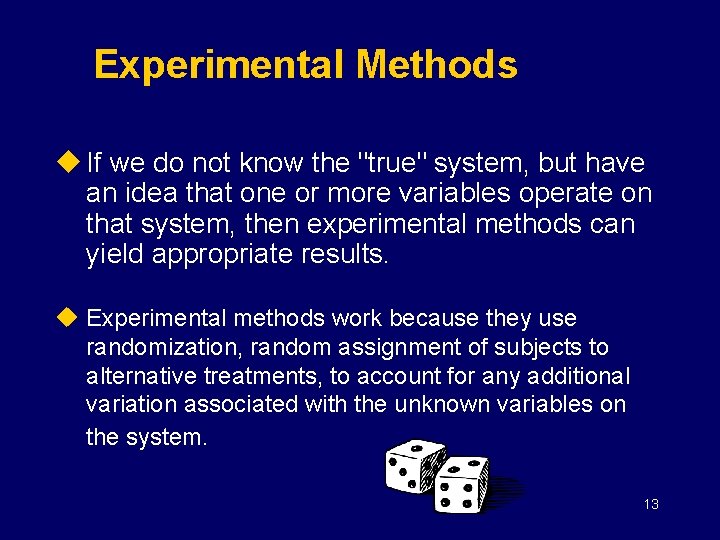
Experimental Methods u If we do not know the "true" system, but have an idea that one or more variables operate on that system, then experimental methods can yield appropriate results. u Experimental methods work because they use randomization, random assignment of subjects to alternative treatments, to account for any additional variation associated with the unknown variables on the system. 13

Observational Data In the case where no experimental control is used in the generation of our data, such data are said to be observational (non-experimental). 14

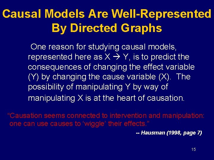
Causal Models Are Well-Represented By Directed Graphs One reason for studying causal models, represented here as X Y, is to predict the consequences of changing the effect variable (Y) by changing the cause variable (X). The possibility of manipulating Y by way of manipulating X is at the heart of causation. “Causation seems connected to intervention and manipulation: one can use causes to ‘wiggle’ their effects. ” -- Hausman (1998, page 7) 15

Directed Acyclic Graphs u Pictures summarizing the causal flow among variables -- there are no cycles. u Inference on causation is informed by asymmetries among causal chains, causal forks, and causal inverted forks. 16

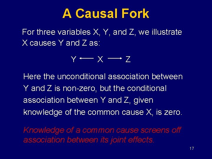
A Causal Fork For three variables X, Y, and Z, we illustrate X causes Y and Z as: Y X Z Here the unconditional association between Y and Z is non-zero, but the conditional association between Y and Z, given knowledge of the common cause X, is zero. Knowledge of a common cause screens off association between its joint effects. 17

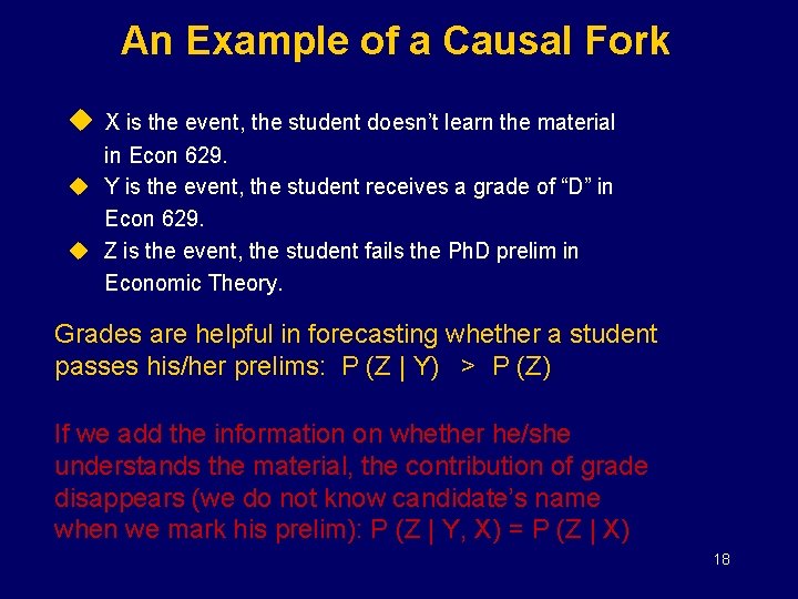
An Example of a Causal Fork u X is the event, the student doesn’t learn the material in Econ 629. u Y is the event, the student receives a grade of “D” in Econ 629. u Z is the event, the student fails the Ph. D prelim in Economic Theory. Grades are helpful in forecasting whether a student passes his/her prelims: P (Z | Y) > P (Z) If we add the information on whether he/she understands the material, the contribution of grade disappears (we do not know candidate’s name when we mark his prelim): P (Z | Y, X) = P (Z | X) 18

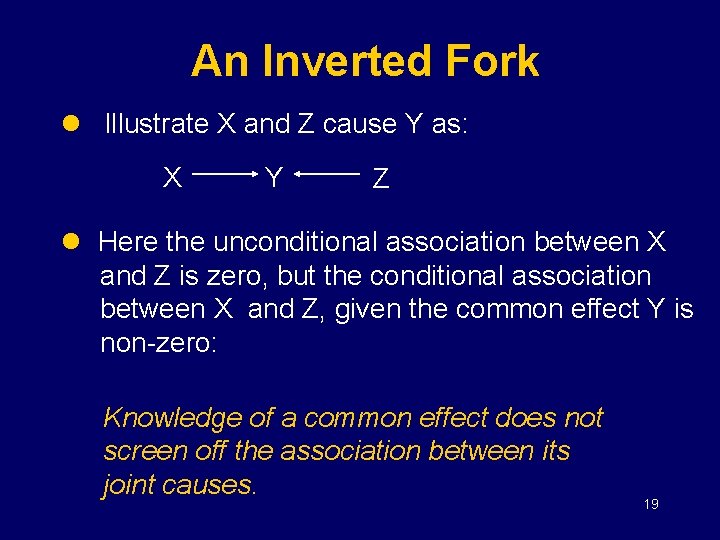
An Inverted Fork l Illustrate X and Z cause Y as: X Y Z l Here the unconditional association between X and Z is zero, but the conditional association between X and Z, given the common effect Y is non-zero: Knowledge of a common effect does not screen off the association between its joint causes. 19

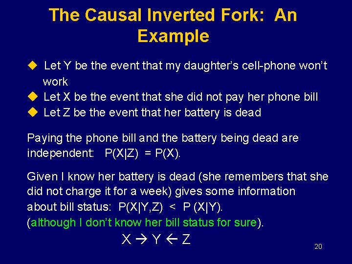
The Causal Inverted Fork: An Example u Let Y be the event that my daughter’s cell-phone won’t work u Let X be the event that she did not pay her phone bill u Let Z be the event that her battery is dead Paying the phone bill and the battery being dead are independent: P(X|Z) = P(X). Given I know her battery is dead (she remembers that she did not charge it for a week) gives some information about bill status: P(X|Y, Z) < P (X|Y). (although I don’t know her bill status for sure). X Y Z 20

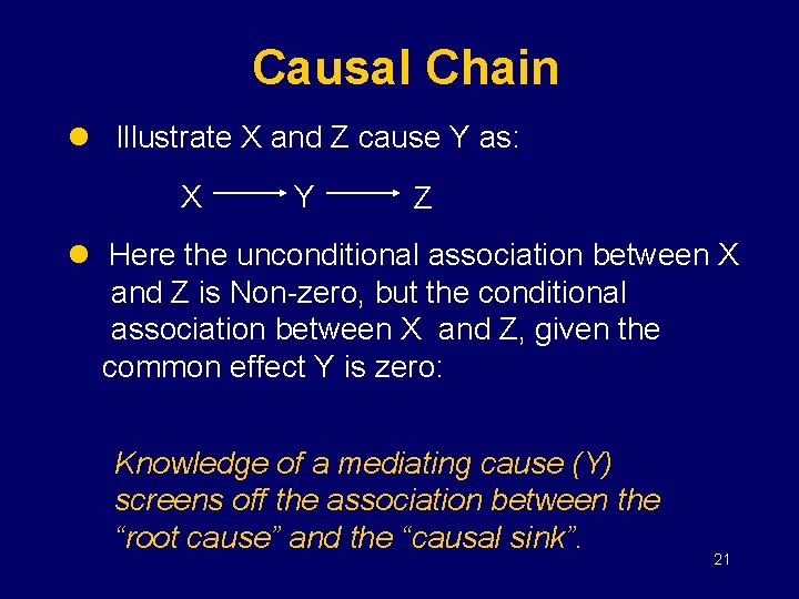
Causal Chain l Illustrate X and Z cause Y as: X Y Z l Here the unconditional association between X and Z is Non-zero, but the conditional association between X and Z, given the common effect Y is zero: Knowledge of a mediating cause (Y) screens off the association between the “root cause” and the “causal sink”. 21

Causal Chains and Time Series Modeling • Possibly the best illustration of use of the correlation structure to identify causal chains is the work of Box and Jenkins: Time series Analysis: Forecasting and Control, Addison Wesley, 1976. • The “tailing off” behavior of the autocorrelation function and the “cutting-off” behavior of the partial autocorrelation function illustrate well these screening off properties of the causal chain. 22

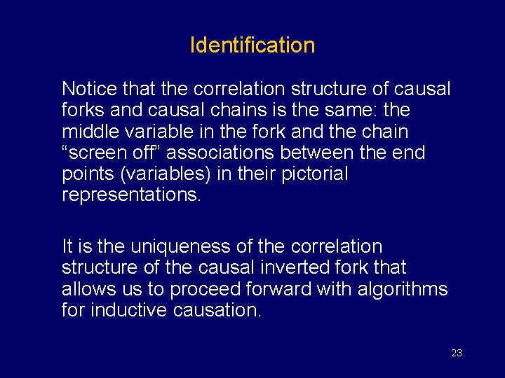
Identification Notice that the correlation structure of causal forks and causal chains is the same: the middle variable in the fork and the chain “screen off” associations between the end points (variables) in their pictorial representations. It is the uniqueness of the correlation structure of the causal inverted fork that allows us to proceed forward with algorithms for inductive causation. 23

The Literature on Such Causal Structures Has Been Advanced in the Last Decade Under the Label of Artificial Intelligence u Pearl , Biometrika, 1995 u Pearl, Causality, Cambridge Press, 2000 u Spirtes, Glymour and Scheines, Causation, Prediction and Search, MIT Press, 2000 u Glymour and Cooper, editors, Computation, Causation and Discovery, MIT Press, 1999 24

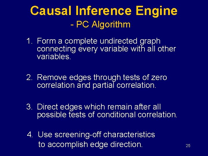
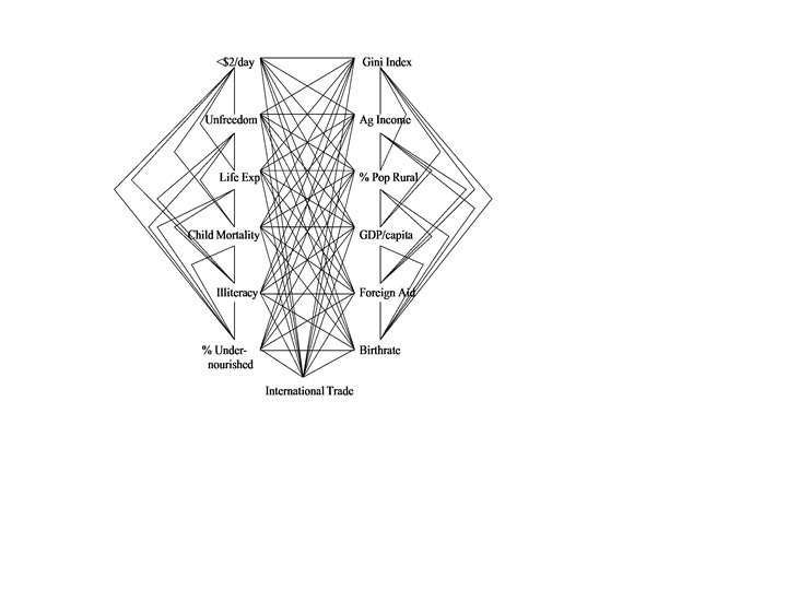
Causal Inference Engine - PC Algorithm 1. Form a complete undirected graph connecting every variable with all other variables. 2. Remove edges through tests of zero correlation and partial correlation. 3. Direct edges which remain after all possible tests of conditional correlation. 4. Use screening-off characteristics to accomplish edge direction. 25

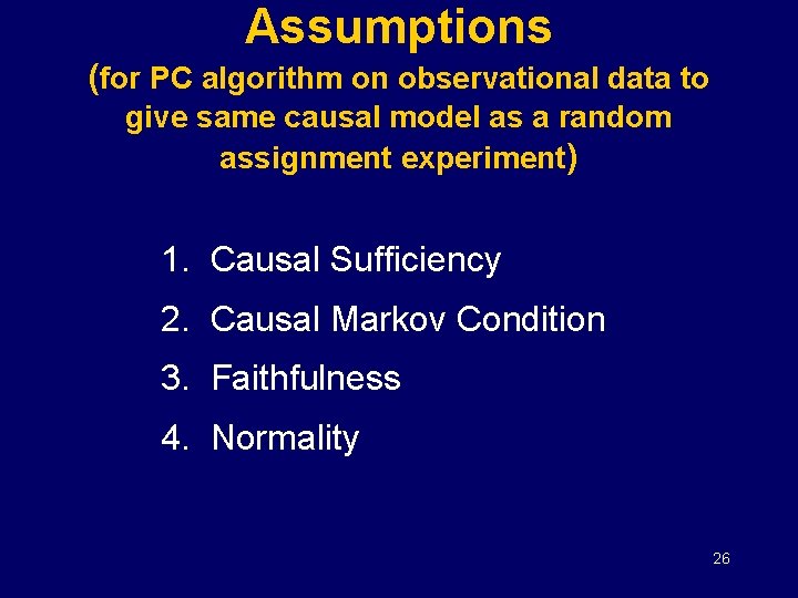
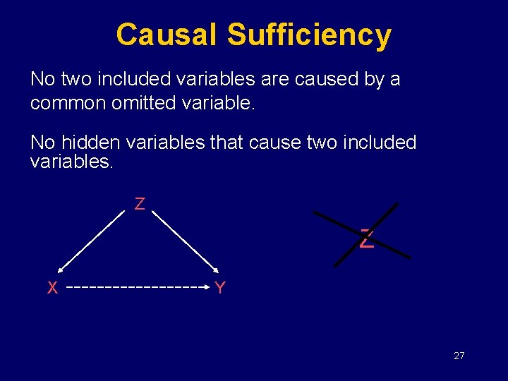
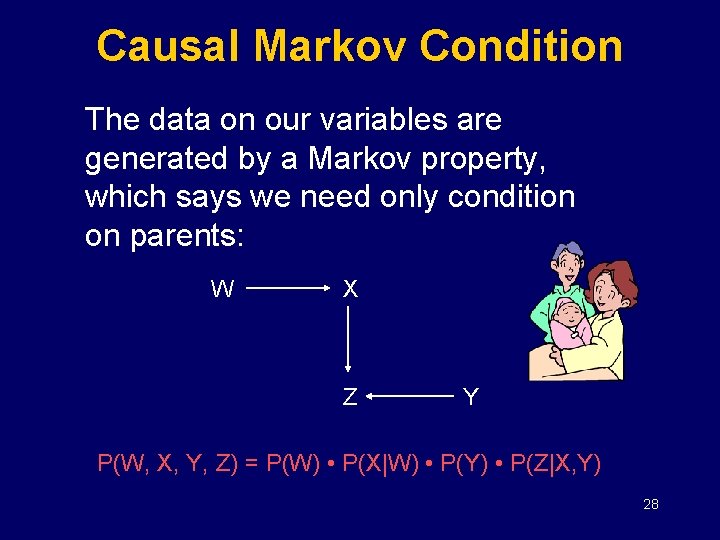
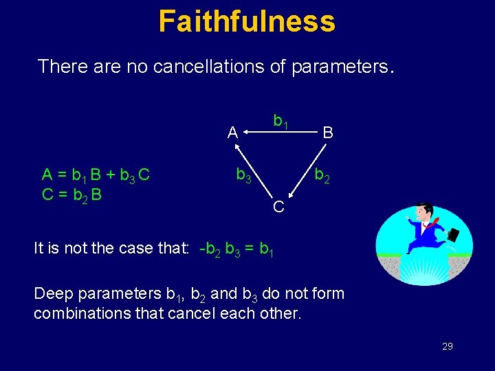
Assumptions (for PC algorithm on observational data to give same causal model as a random assignment experiment) 1. Causal Sufficiency 2. Causal Markov Condition 3. Faithfulness 4. Normality 26

Causal Sufficiency No two included variables are caused by a common omitted variable. No hidden variables that cause two included variables. Z Z X Y 27

Causal Markov Condition The data on our variables are generated by a Markov property, which says we need only condition on parents: W X Z Y P(W, X, Y, Z) = P(W) • P(X|W) • P(Y) • P(Z|X, Y) 28

Faithfulness There are no cancellations of parameters. A A = b 1 B + b 3 C C = b 2 B b 1 b 3 B b 2 C It is not the case that: -b 2 b 3 = b 1 Deep parameters b 1, b 2 and b 3 do not form combinations that cancel each other. 29

30

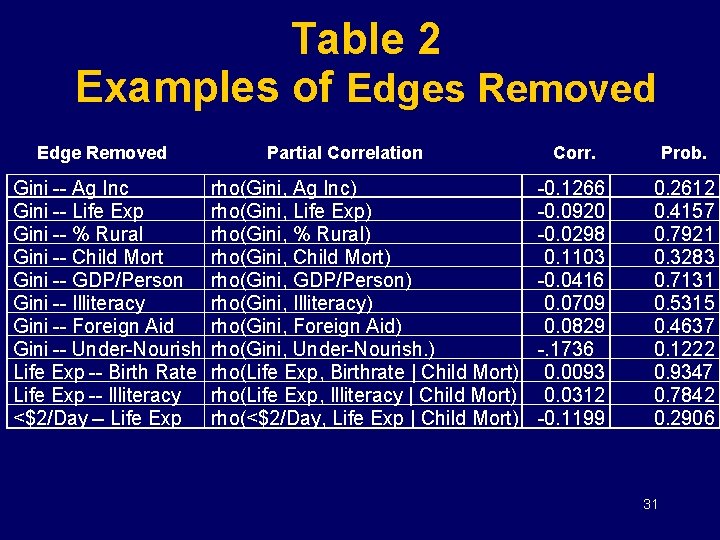
Table 2 Examples of Edges Removed Edge Removed Gini -- Ag Inc Gini -- Life Exp Gini -- % Rural Gini -- Child Mort Gini -- GDP/Person Gini -- Illiteracy Gini -- Foreign Aid Gini -- Under-Nourish Life Exp -- Birth Rate Life Exp -- Illiteracy <$2/Day -- Life Exp Partial Correlation rho(Gini, Ag Inc) rho(Gini, Life Exp) rho(Gini, % Rural) rho(Gini, Child Mort) rho(Gini, GDP/Person) rho(Gini, Illiteracy) rho(Gini, Foreign Aid) rho(Gini, Under-Nourish. ) rho(Life Exp, Birthrate | Child Mort) rho(Life Exp, Illiteracy | Child Mort) rho(<$2/Day, Life Exp | Child Mort) Corr. Prob. -0. 1266 -0. 0920 -0. 0298 0. 1103 -0. 0416 0. 0709 0. 0829 -. 1736 0. 0093 0. 0312 -0. 1199 0. 2612 0. 4157 0. 7921 0. 3283 0. 7131 0. 5315 0. 4637 0. 1222 0. 9347 0. 7842 0. 2906 31

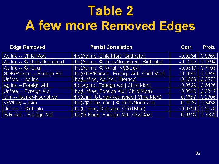
Table 2 A few more Removed Edges Edge Removed Ag Inc -- Child Mort Ag Inc -- % Undr-Nourished Ag Inc -- % Rural GDP/Person -- Foreign Aid Unfree -- Ag Inc – Foreign Aid Unfree -- Foreign Aid Gini -- %Undr-Nourished <$2/Day -- Gini Unfree -- Birthrate % Rural -- Foreign Aid Partial Correlation rho(Ag Inc, Child Mort | Birthrate) rho(Ag Inc, % Undr-Nourished | Birthrate) rho(Ag Inc, % Rural | <$2/Day) rho(GDP/Person, Foreign Aid | Child Mort) rho(Unfree, Ag Inc | Illiteracy) rho(Ag Inc, Foreign Aid | Child Mort) rho(Unfree, Foreign Aid | Child Mort) rho(Gini, % Undr-Nourished | Child Mort) rho(<$2/Day, Gini | % Undr-Nourised) rho(Unfree, Birthrate | Child Mort) rho(% Rural, Foreig n Aid | <$2/Day) Corr. Prob. -0. 0234 -0. 1202 -0. 0319 -0. 1096 -0. 1368 -0. 0529 -0. 0546 0. 1357 0. 1075 -0. 0754 0. 0313 0. 8369 0. 2894 0. 7793 0. 3344 0. 2272 0. 6426 0. 6317 0. 2306 0. 3438 0. 5078 0. 7832 32

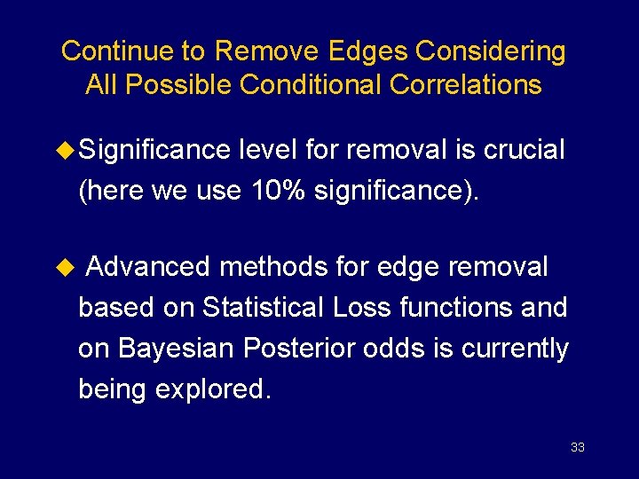
Continue to Remove Edges Considering All Possible Conditional Correlations u Significance level for removal is crucial (here we use 10% significance). u Advanced methods for edge removal based on Statistical Loss functions and on Bayesian Posterior odds is currently being explored. 33

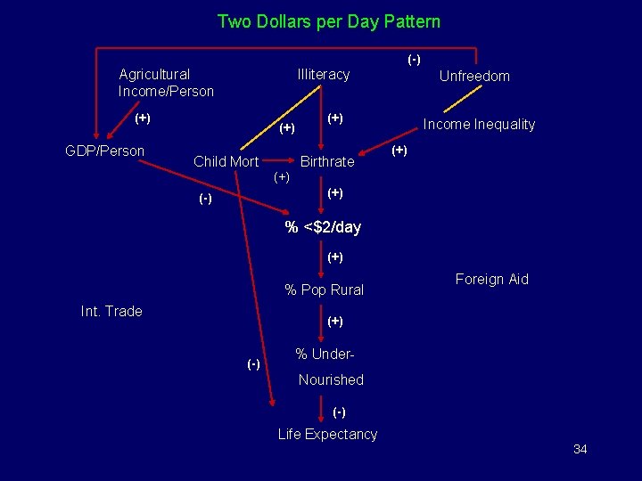
Two Dollars per Day Pattern (-) Agricultural Income/Person Illiteracy (+) GDP/Person (+) Child Mort Unfreedom (+) Birthrate Income Inequality (+) (+) (-) % <$2/day (+) % Pop Rural Int. Trade Foreign Aid (+) (-) % Under. Nourished (-) Life Expectancy 34

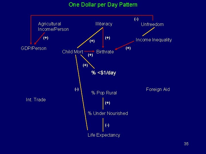
One Dollar per Day Pattern (-) Agricultural Income/Person Illiteracy (+) GDP/Person (+) Child Mort (+) Unfreedom (+) Birthrate Income Inequality (+) % <$1/day (-) Int. Trade % Pop Rural Foreign Aid (+) % Under Nourished (-) Life Expectancy 35

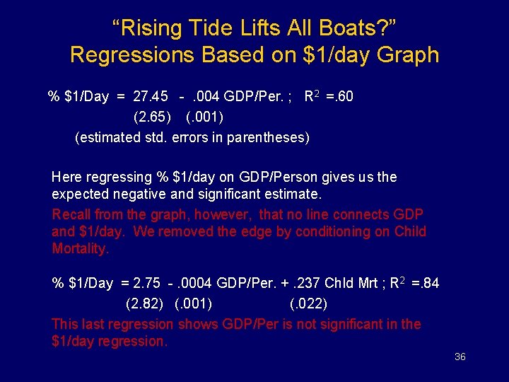
“Rising Tide Lifts All Boats? ” Regressions Based on $1/day Graph % $1/Day = 27. 45 -. 004 GDP/Per. ; R 2 =. 60 (2. 65) (. 001) (estimated std. errors in parentheses) Here regressing % $1/day on GDP/Person gives us the expected negative and significant estimate. Recall from the graph, however, that no line connects GDP and $1/day. We removed the edge by conditioning on Child Mortality. % $1/Day = 2. 75 -. 0004 GDP/Per. +. 237 Chld Mrt ; R 2 =. 84 (2. 82) (. 001) (. 022) This last regression shows GDP/Per is not significant in the $1/day regression. 36

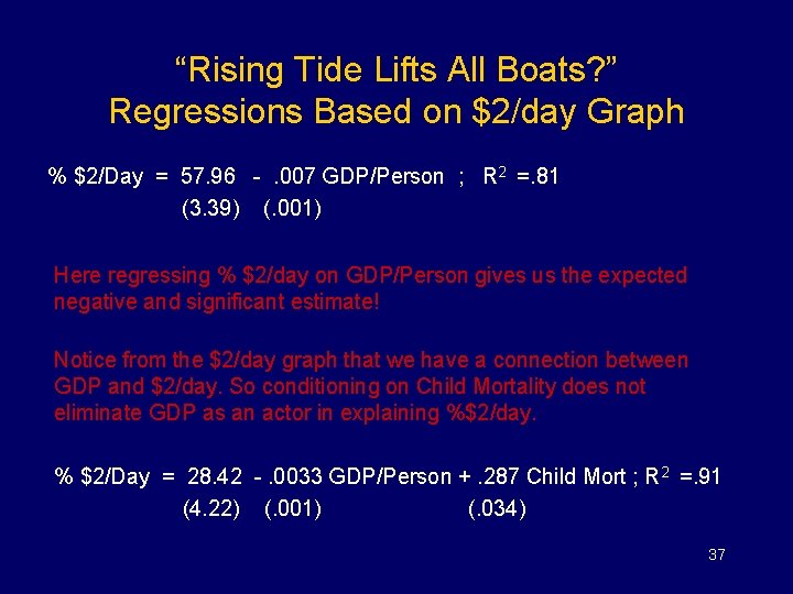
“Rising Tide Lifts All Boats? ” Regressions Based on $2/day Graph % $2/Day = 57. 96 -. 007 GDP/Person ; R 2 =. 81 (3. 39) (. 001) Here regressing % $2/day on GDP/Person gives us the expected negative and significant estimate! Notice from the $2/day graph that we have a connection between GDP and $2/day. So conditioning on Child Mortality does not eliminate GDP as an actor in explaining %$2/day. % $2/Day = 28. 42 -. 0033 GDP/Person +. 287 Child Mort ; R 2 =. 91 (4. 22) (. 001) (. 034) 37

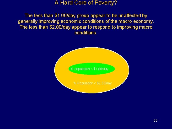
A Hard Core of Poverty? The less than $1. 00/day group appear to be unaffected by generally improving economic conditions of the macro economy. The less than $2. 00/day appear to respond to improving macro conditions. % population < $1. 00/day % Population < $2. 00/day 38

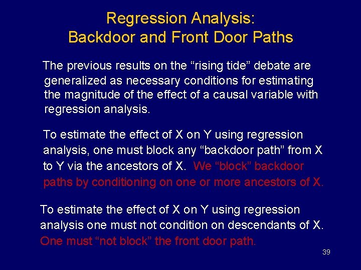
Regression Analysis: Backdoor and Front Door Paths The previous results on the “rising tide” debate are generalized as necessary conditions for estimating the magnitude of the effect of a causal variable with regression analysis. To estimate the effect of X on Y using regression analysis, one must block any “backdoor path” from X to Y via the ancestors of X. We “block” backdoor paths by conditioning on one or more ancestors of X. To estimate the effect of X on Y using regression analysis one must not condition on descendants of X. One must “not block” the front door path. 39

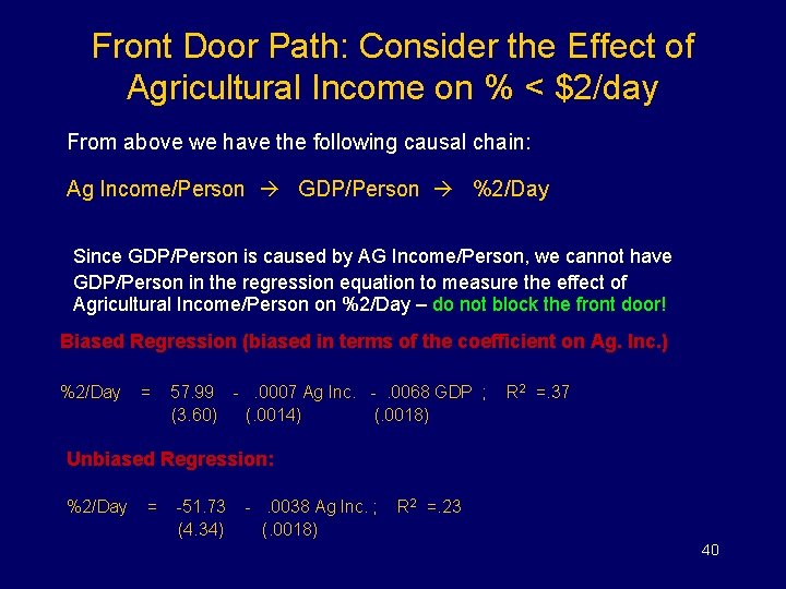
Front Door Path: Consider the Effect of Agricultural Income on % < $2/day From above we have the following causal chain: Ag Income/Person GDP/Person %2/Day Since GDP/Person is caused by AG Income/Person, we cannot have GDP/Person in the regression equation to measure the effect of Agricultural Income/Person on %2/Day – do not block the front door! Biased Regression (biased in terms of the coefficient on Ag. Inc. ) %2/Day = 57. 99 -. 0007 Ag Inc. -. 0068 GDP ; (3. 60) (. 0014) (. 0018) R 2 =. 37 Unbiased Regression: %2/Day = -51. 73 (4. 34) -. 0038 Ag Inc. ; (. 0018) R 2 =. 23 40

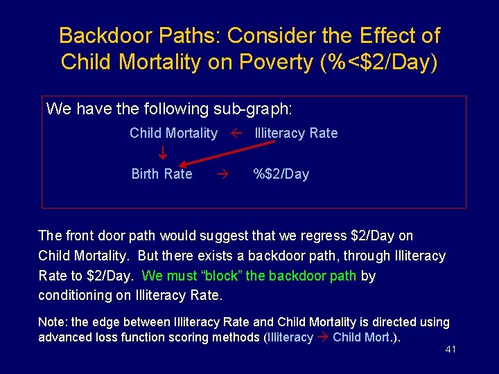
Backdoor Paths: Consider the Effect of Child Mortality on Poverty (%<$2/Day) We have the following sub-graph: Child Mortality Illiteracy Rate Birth Rate %$2/Day The front door path would suggest that we regress $2/Day on Child Mortality. But there exists a backdoor path, through Illiteracy Rate to $2/Day. We must “block” the backdoor path by conditioning on Illiteracy Rate. Note: the edge between Illiteracy Rate and Child Mortality is directed using advanced loss function scoring methods (Illiteracy Child Mort. ). 41

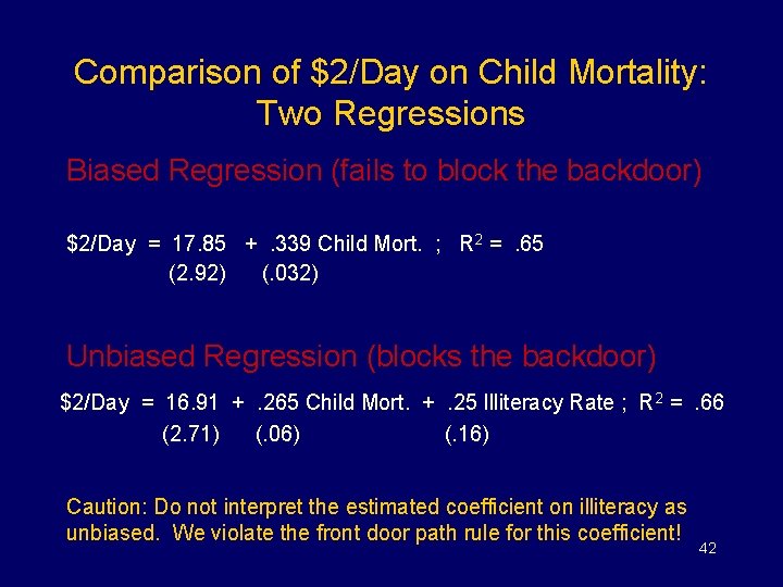
Comparison of $2/Day on Child Mortality: Two Regressions Biased Regression (fails to block the backdoor) $2/Day = 17. 85 +. 339 Child Mort. ; R 2 =. 65 (2. 92) (. 032) Unbiased Regression (blocks the backdoor) $2/Day = 16. 91 +. 265 Child Mort. +. 25 Illiteracy Rate ; R 2 =. 66 (2. 71) (. 06) (. 16) Caution: Do not interpret the estimated coefficient on illiteracy as unbiased. We violate the front door path rule for this coefficient! 42

Conclusions Given our set of variables: Illiteracy, Freedom, and Agricultural Income are exogenous movers of (root causes of) poverty. Given the assumptions in the directed graphs literature, we can consider manipulations of poverty by manipulations in one or more of these causes. Whether or not any of these can be “easily” manipulated is, of course, another question. Use of regression techniques to measure the quantitative relationship between causes and effects requires that we block backdoor paths and not block front door paths. 43

Caution Our methods assume: u Causal Sufficiency u Markov Property u Faithfulness u Normality Failure of any of these may change results. 44

More Caution: Duhem’s Thesis Foreign Aid may be better measured (for our purposes) as Foreign Aid for Poverty Alleviation (the variable we use is Total Foreign Aid). International trade might well be measured without natural resource exports (Dutch Disease). Dynamic representation of poverty should be pursued. This will require a richer data set. 45

Acknowledgements Motivation for the study Aysen Tanyeri-Abur, FAO Motivation for our study of Directed Graphs Clark Glymour, CMU Judea Pearl, UCLA 46