Direct Volume Rendering Acknowledgement HanWei Shen Lecture Notes

Direct Volume Rendering Acknowledgement : Han-Wei Shen Lecture Notes 사용

Direct Volume Rendering • Direct : no conversion to surface geometry • Three methods – Ray-Casting – Splatting – 3 D Texture-Based Method

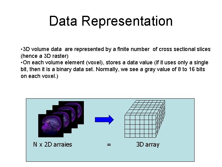
Data Representation • 3 D volume data are represented by a finite number of cross sectional slices (hence a 3 D raster) • On each volume element (voxel), stores a data value (if it uses only a single bit, then it is a binary data set. Normally, we see a gray value of 8 to 16 bits on each voxel. ) N x 2 D arraies = 3 D array

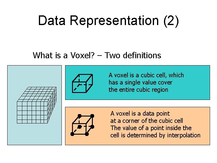
Data Representation (2) What is a Voxel? – Two definitions A voxel is a cubic cell, which has a single value cover the entire cubic region A voxel is a data point at a corner of the cubic cell The value of a point inside the cell is determined by interpolation

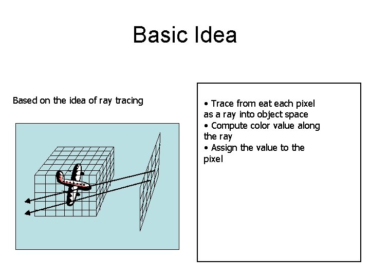
Basic Idea Based on the idea of ray tracing • Trace from eat each pixel as a ray into object space • Compute color value along the ray • Assign the value to the pixel

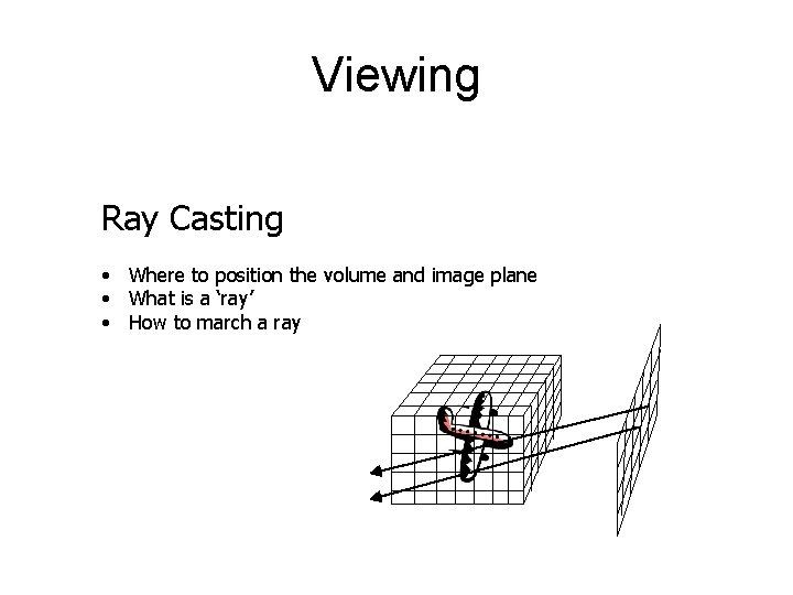
Viewing Ray Casting • Where to position the volume and image plane • What is a ‘ray’ • How to march a ray

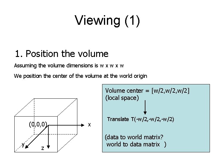
Viewing (1) 1. Position the volume Assuming the volume dimensions is w x w We position the center of the volume at the world origin Volume center = [w/2, w/2] (local space) (0, 0, 0) y z x Translate T(-w/2, -w/2) (data to world matrix? world to data matrix )

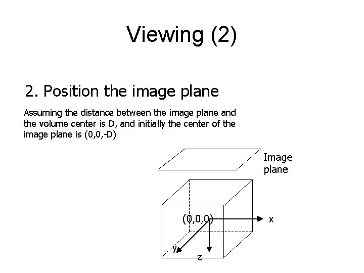
Viewing (2) 2. Position the image plane Assuming the distance between the image plane and the volume center is D, and initially the center of the image plane is (0, 0, -D) Image plane (0, 0, 0) y z x

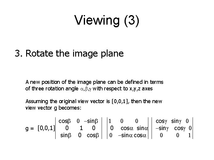
Viewing (3) 3. Rotate the image plane A new position of the image plane can be defined in terms of three rotation angle , b, g with respect to x, y, z axes Assuming the original view vector is [0, 0, 1], then the new view vector g becomes: cosb 0 -sinb g = [0, 0, 1] 0 1 0 sinb 0 cosb 1 0 0 0 cos sin 0 -sin cosg sing 0 -sing cosg 0 0 0 1

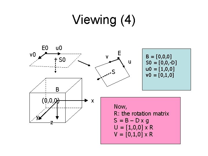
Viewing (4) E 0 v 0 u 0 E v + S 0 u S B = [0, 0, 0] S 0 = [0, 0, -D] u 0 = [1, 0, 0] v 0 = [0, 1, 0] B (0, 0, 0) y z x Now, R: the rotation matrix S=B–Dxg U = [1, 0, 0] x R V = [0, 1, 0] x R

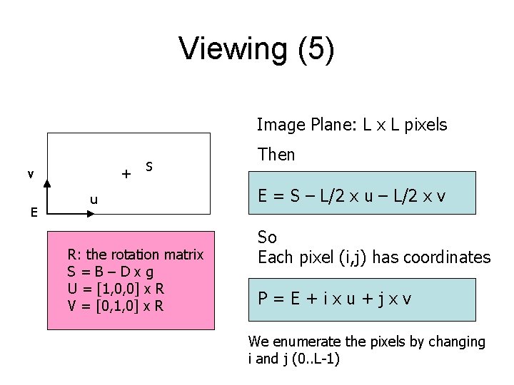
Viewing (5) Image Plane: L x L pixels + v E S u R: the rotation matrix S=B–Dxg U = [1, 0, 0] x R V = [0, 1, 0] x R Then E = S – L/2 x u – L/2 x v So Each pixel (i, j) has coordinates P=E+ixu+jxv We enumerate the pixels by changing i and j (0. . L-1)

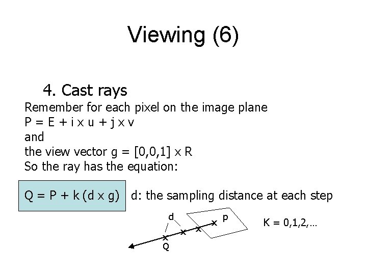
Viewing (6) 4. Cast rays Remember for each pixel on the image plane P=E+ixu+jxv and the view vector g = [0, 0, 1] x R So the ray has the equation: Q = P + k (d x g) d: the sampling distance at each step d x Q x x x p K = 0, 1, 2, …

Old Methods • Before 1988 • Did not consider transparency • did not consider sophisticated light transportation theory • were concerned with quick solutions • hence more or less applied to binary data non-binary data require sophisticated classification/compositing methods!

Ray Tracing -> Ray Casting • “another” typical method from traditional graphics • Typically we only deal with primary rays hence: ray-casting • a natural image-order technique • as opposed to surface graphics - how do we calculate the ray/surface intersection? ? ? • Since we have no surfaces - we need to carefully step through the volume

Ray Casting • Stepping through the volume: a ray is cast into the volume, sampling the volume at certain intervals • The sampling intervals are usually equi-distant, but don’t have to be (e. g. importance sampling) • At each sampling location, a sample is interpolated / reconstructed from the grid voxels • popular filters are: nearest neighbor (box), trilinear (tent), Gaussian, cubic spline • Along the ray - what are we looking for?

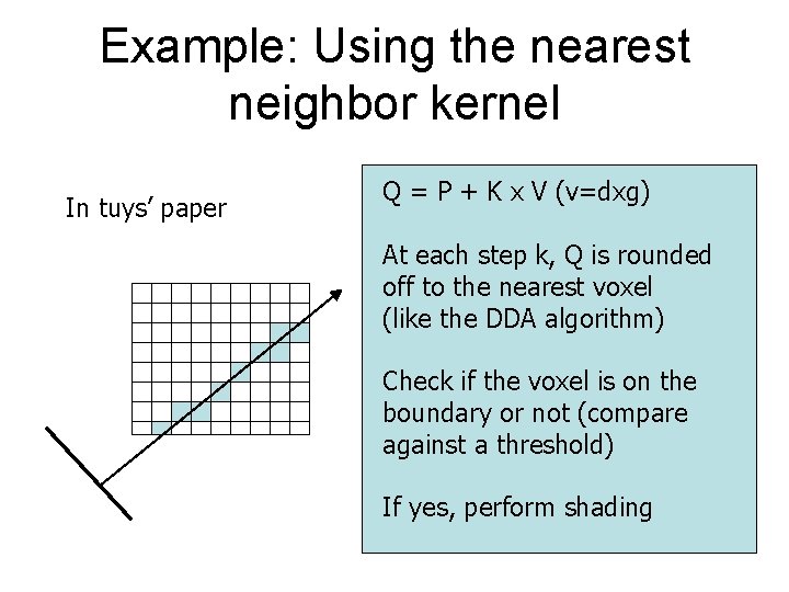
Example: Using the nearest neighbor kernel In tuys’ paper Q = P + K x V (v=dxg) At each step k, Q is rounded off to the nearest voxel (like the DDA algorithm) Check if the voxel is on the boundary or not (compare against a threshold) If yes, perform shading

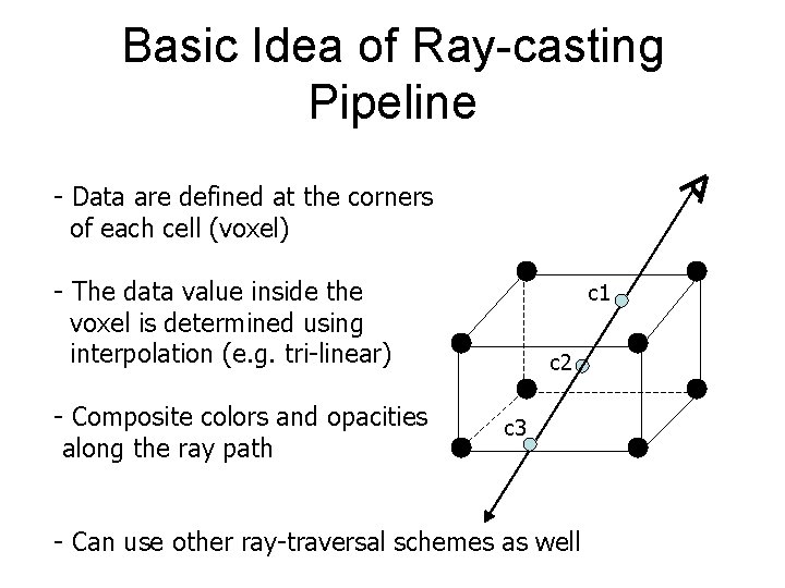
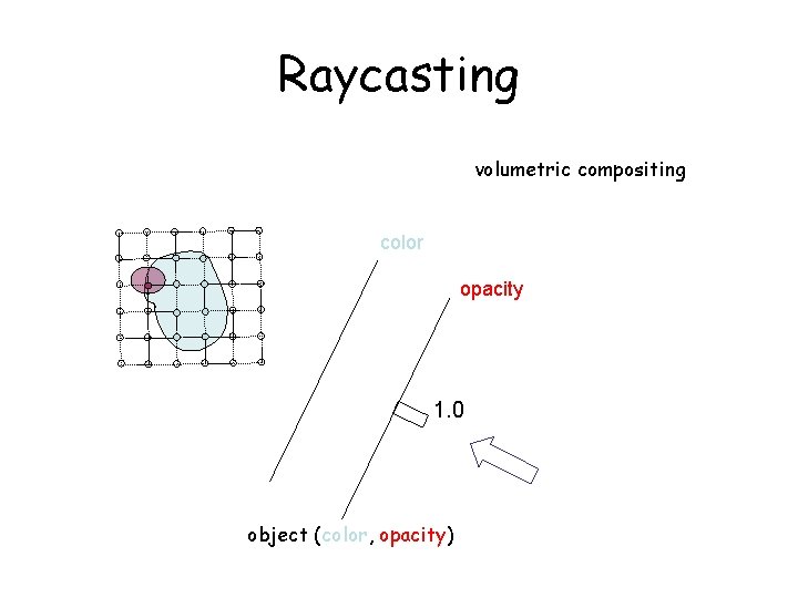
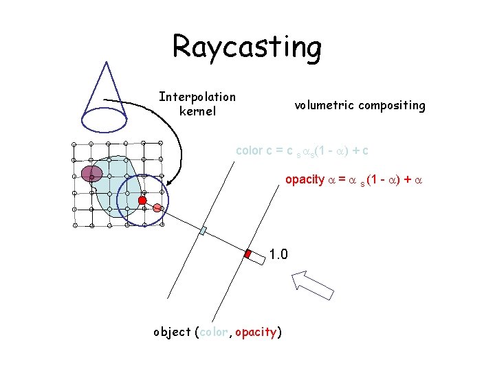
Basic Idea of Ray-casting Pipeline - Data are defined at the corners of each cell (voxel) - The data value inside the voxel is determined using interpolation (e. g. tri-linear) - Composite colors and opacities along the ray path c 1 c 2 c 3 - Can use other ray-traversal schemes as well

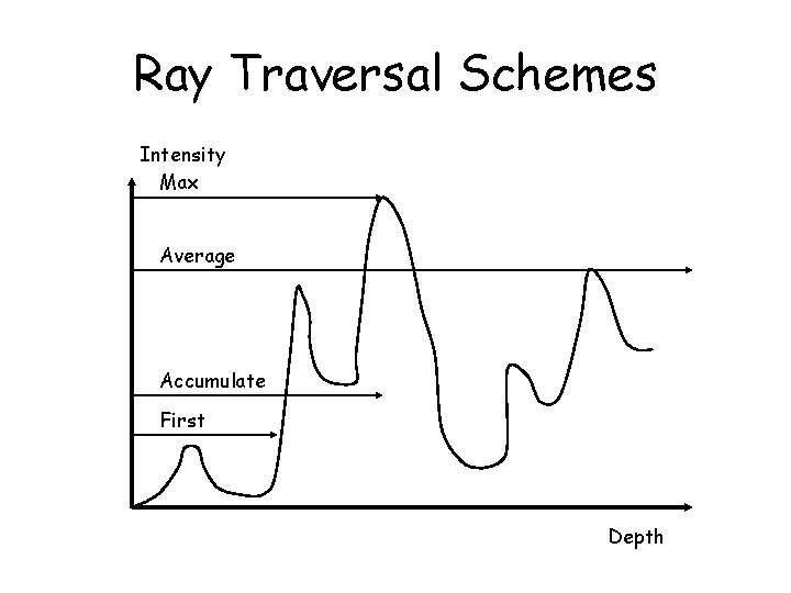
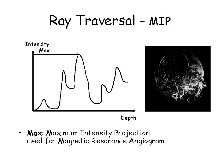
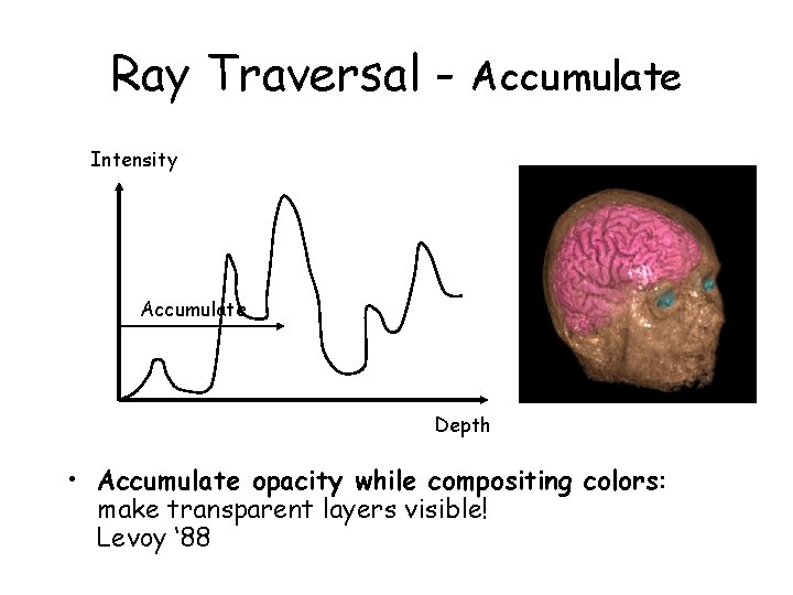
Ray Traversal Schemes Intensity Max Average Accumulate First Depth

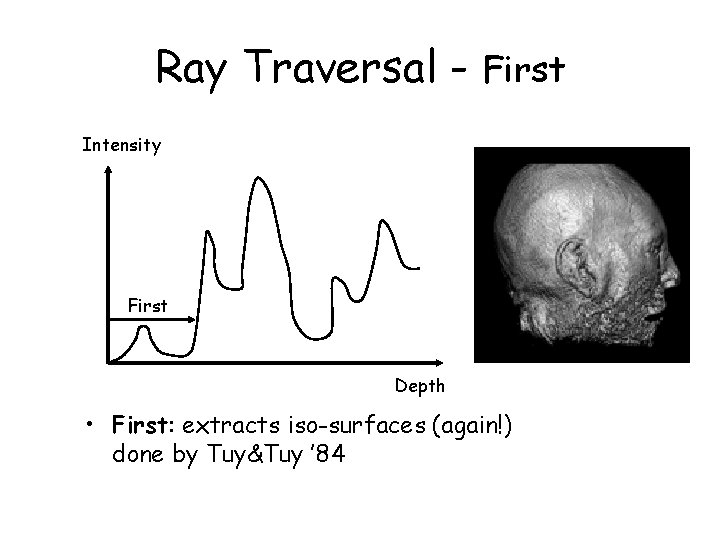
Ray Traversal - First Intensity First Depth • First: extracts iso-surfaces (again!) done by Tuy&Tuy ’ 84

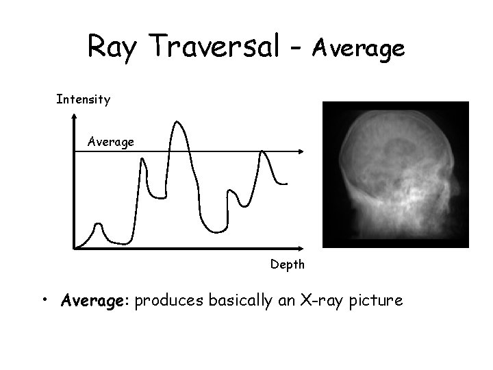
Ray Traversal - Average Intensity Average Depth • Average: produces basically an X-ray picture

Ray Traversal - MIP Intensity Max Depth • Max: Maximum Intensity Projection used for Magnetic Resonance Angiogram

Ray Traversal - Accumulate Intensity Accumulate Depth • Accumulate opacity while compositing colors: make transparent layers visible! Levoy ‘ 88

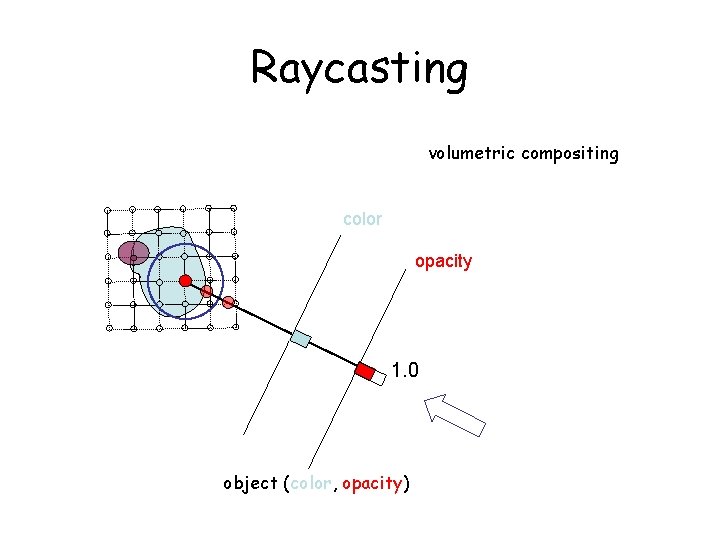
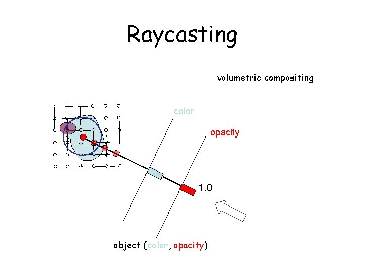
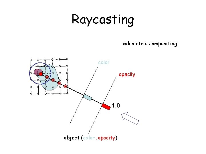
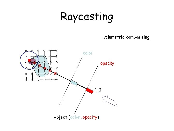
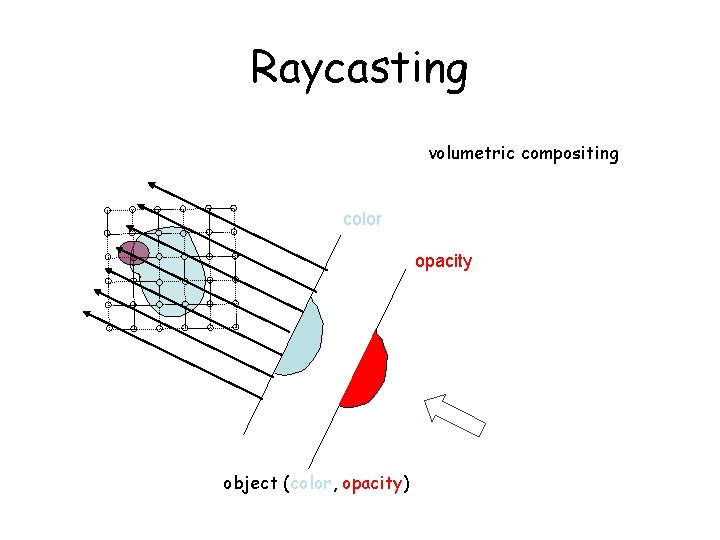
Raycasting volumetric compositing color opacity 1. 0 object (color, opacity)

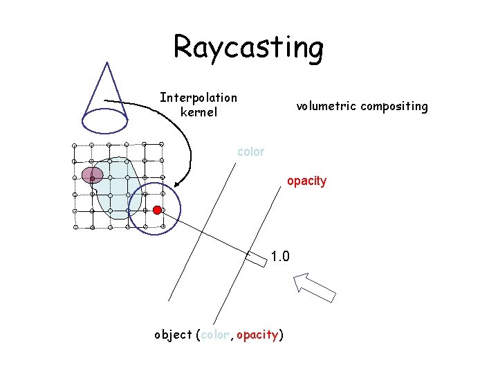
Raycasting Interpolation kernel volumetric compositing color opacity 1. 0 object (color, opacity)

Raycasting Interpolation kernel volumetric compositing color c = c s s(1 - ) + c opacity = s (1 - ) + 1. 0 object (color, opacity)

Raycasting volumetric compositing color opacity 1. 0 object (color, opacity)

Raycasting volumetric compositing color opacity 1. 0 object (color, opacity)

Raycasting volumetric compositing color opacity 1. 0 object (color, opacity)

Raycasting volumetric compositing color opacity 1. 0 object (color, opacity)

Raycasting volumetric compositing color opacity object (color, opacity)

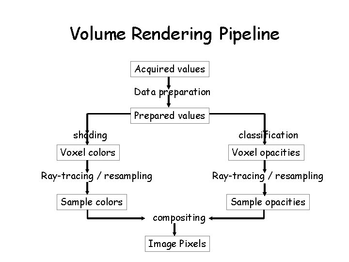
Volume Rendering Pipeline Acquired values Data preparation Prepared values shading classification Voxel colors Voxel opacities Ray-tracing / resampling Sample colors Sample opacities compositing Image Pixels

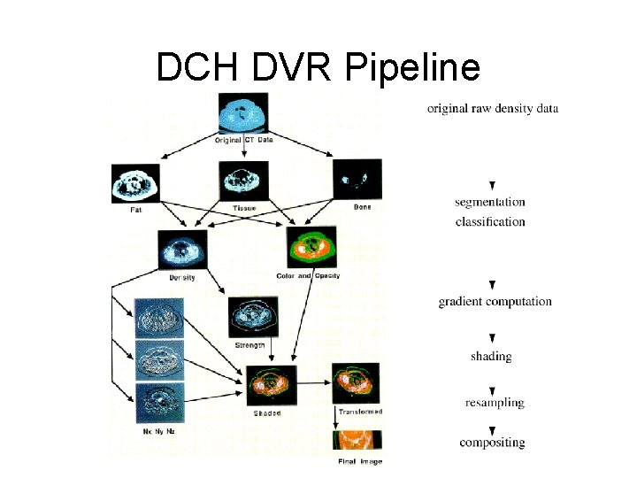
DCH DVR Pipeline

Common Components of General Pipeline • Interpolation/reconstruction • Classification or transfer function • Gradient/normal estimation for shading – Question: are normals also interpolated?

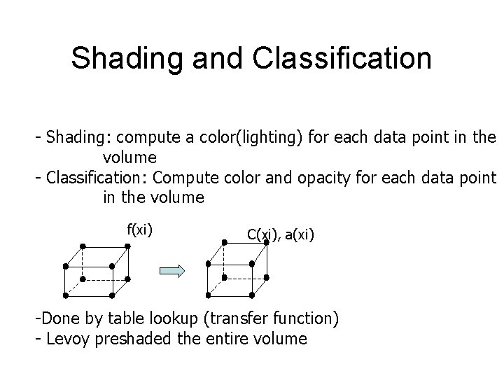
Shading and Classification - Shading: compute a color(lighting) for each data point in the volume - Classification: Compute color and opacity for each data point in the volume f(xi) C(xi), a(xi) -Done by table lookup (transfer function) - Levoy preshaded the entire volume

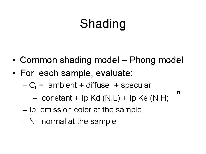
Shading • Common shading model – Phong model • For each sample, evaluate: – Ci = ambient + diffuse + specular = constant + Ip Kd (N. L) + Ip Ks (N. H) – Ip: emission color at the sample – N: normal at the sample n

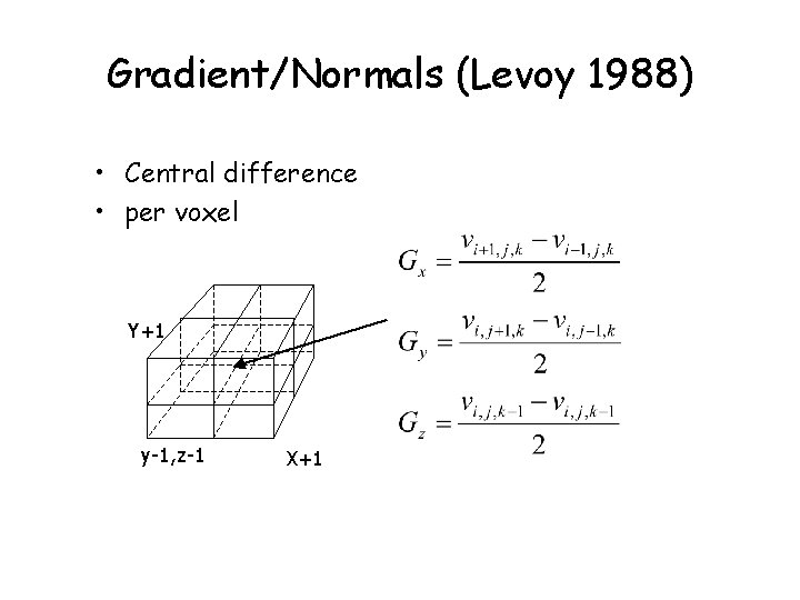
Gradient/Normals (Levoy 1988) • Central difference • per voxel Y+1 y-1, z-1 X+1

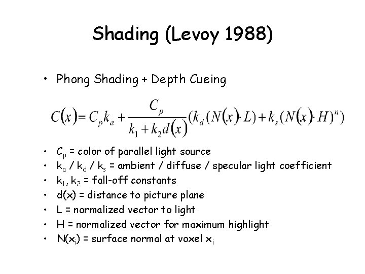
Shading (Levoy 1988) • Phong Shading + Depth Cueing • • Cp = color of parallel light source ka / kd / ks = ambient / diffuse / specular light coefficient k 1, k 2 = fall-off constants d(x) = distance to picture plane L = normalized vector to light H = normalized vector for maximum highlight N(xi) = surface normal at voxel xi

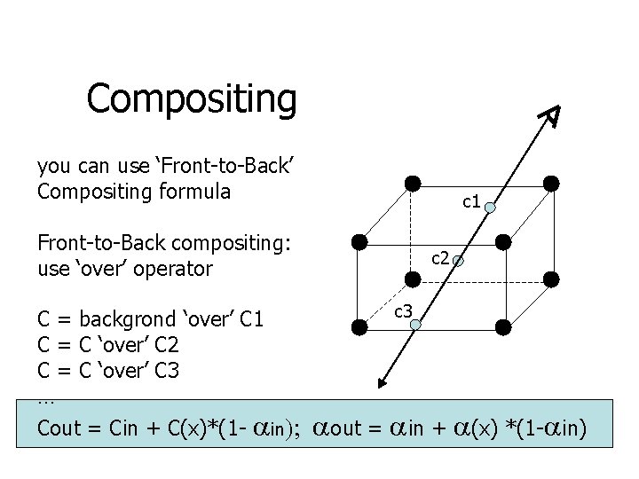
Compositing you can use ‘Front-to-Back’ Compositing formula c 1 Front-to-Back compositing: use ‘over’ operator C = backgrond ‘over’ C 1 C = C ‘over’ C 2 C = C ‘over’ C 3 … Cout = Cin + C(x)*(1 - c 2 c 3 in); out = in + (x) *(1 - in)

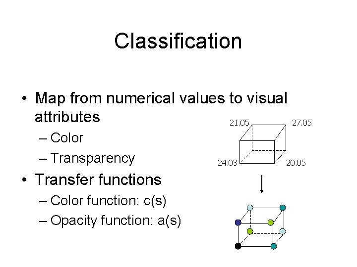
Classification • Map from numerical values to visual attributes 21. 05 27. 05 – Color – Transparency • Transfer functions – Color function: c(s) – Opacity function: a(s) 24. 03 20. 05

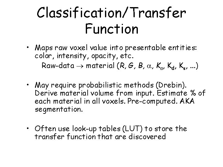
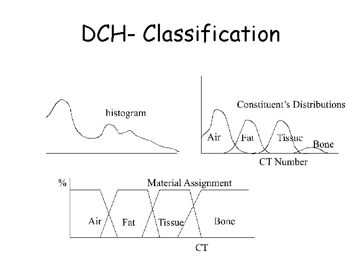
Classification/Transfer Function • Maps raw voxel value into presentable entities: color, intensity, opacity, etc. Raw-data material (R, G, B, , Ka, Kd, Ks, . . . ) • May require probabilistic methods (Drebin). Derive material volume from input. Estimate % of each material in all voxels. Pre-computed. AKA segmentation. • Often use look-up tables (LUT) to store the transfer function that are discovered

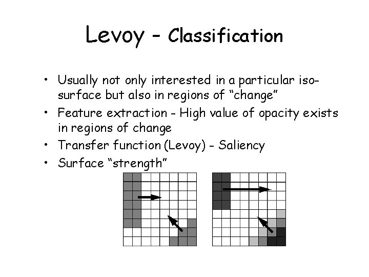
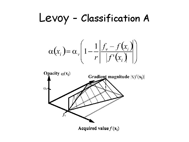
Levoy - Classification • Usually not only interested in a particular isosurface but also in regions of “change” • Feature extraction - High value of opacity exists in regions of change • Transfer function (Levoy) - Saliency • Surface “strength”

Opacity function (1) Goal: visualize voxels that have a selected threshold value fv - No intermediate geometry is extracted - The idea is to assign voxels that have value fv the maximum opacity (say ) - And then create a smooth transition for the surrounding area from 1 to 0 -Levoy wants to maintain a constant thickness for the transition area.

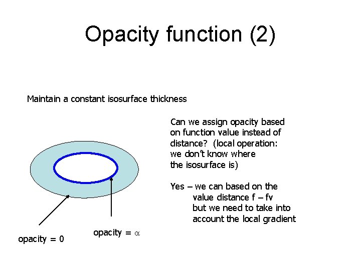
Opacity function (2) Maintain a constant isosurface thickness Can we assign opacity based on function value instead of distance? (local operation: we don’t know where the isosurface is) Yes – we can based on the value distance f – fv but we need to take into account the local gradient opacity = 0 opacity =

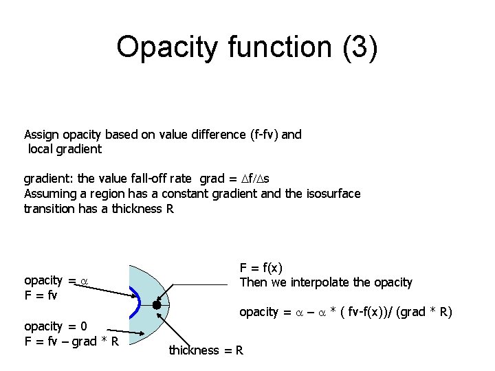
Opacity function (3) Assign opacity based on value difference (f-fv) and local gradient: the value fall-off rate grad = Df/Ds Assuming a region has a constant gradient and the isosurface transition has a thickness R opacity = F = fv opacity = 0 F = fv – grad * R F = f(x) Then we interpolate the opacity = – * ( fv-f(x))/ (grad * R) thickness = R

Levoy - Classification A

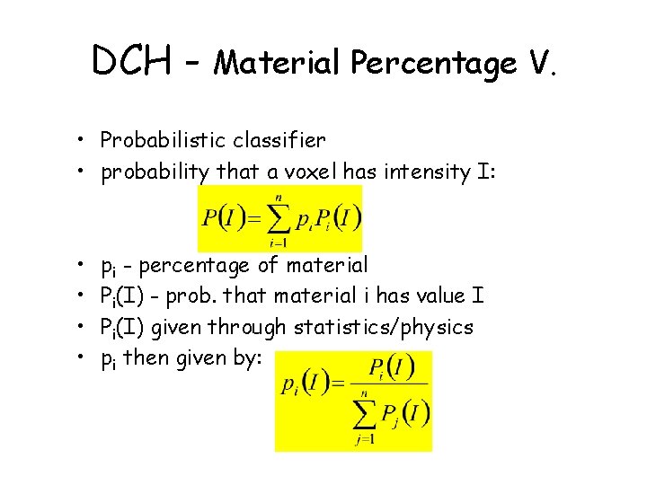
DCH - Material Percentage V. • Probabilistic classifier • probability that a voxel has intensity I: • • pi - percentage of material Pi(I) - prob. that material i has value I Pi(I) given through statistics/physics pi then given by:

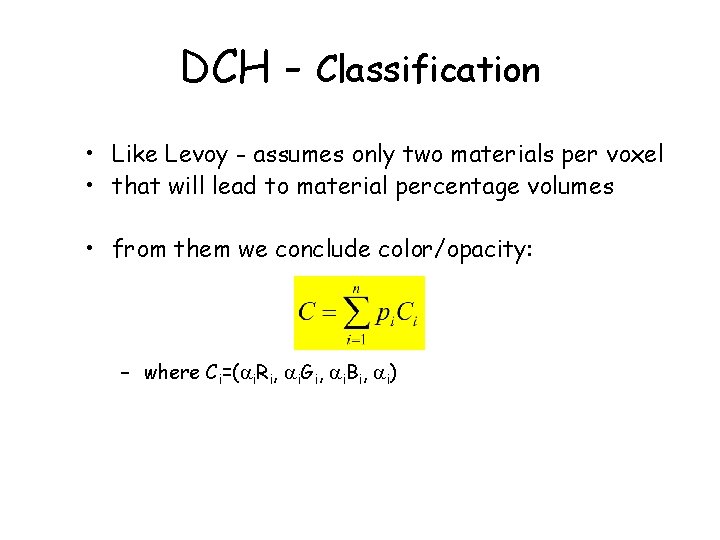
DCH - Classification • Like Levoy - assumes only two materials per voxel • that will lead to material percentage volumes • from them we conclude color/opacity: – where Ci=( i. Ri, i. Gi, i. Bi, i)

DCH- Classification

Levoy - Improvements • Levoy 1990 • front-to-back with early ray termination = 0. 95 • hierarchical oct-tree data structure – skip empty cells efficiently

Texture Based Volume Rendering

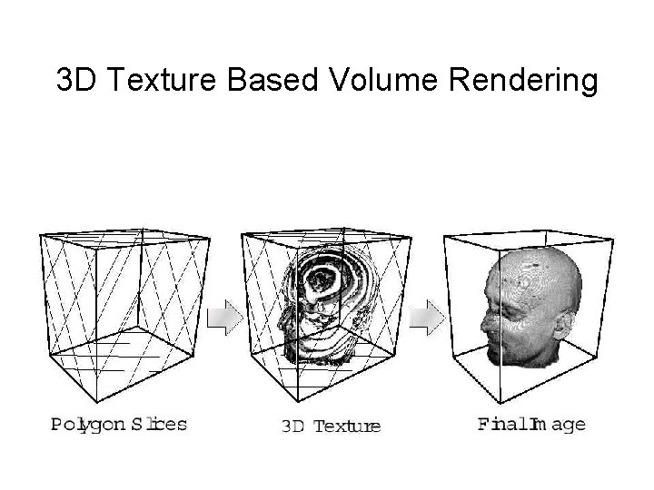
3 D Texture Based Volume Rendering • Best known practical volume rendering method for rectlinear grid datasets • Realtime Rendering is possible

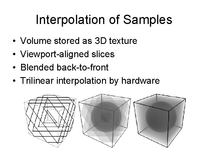
Interpolation of Samples • • Volume stored as 3 D texture Viewport-aligned slices Blended back-to-front Trilinear interpolation by hardware

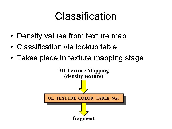
Classification • Density values from texture map • Classification via lookup table • Takes place in texture mapping stage

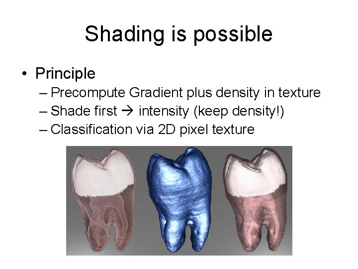
Shading is possible • Principle – Precompute Gradient plus density in texture – Shade first intensity (keep density!) – Classification via 2 D pixel texture

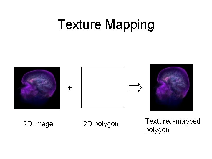
Texture Mapping + 2 D image 2 D polygon Textured-mapped polygon

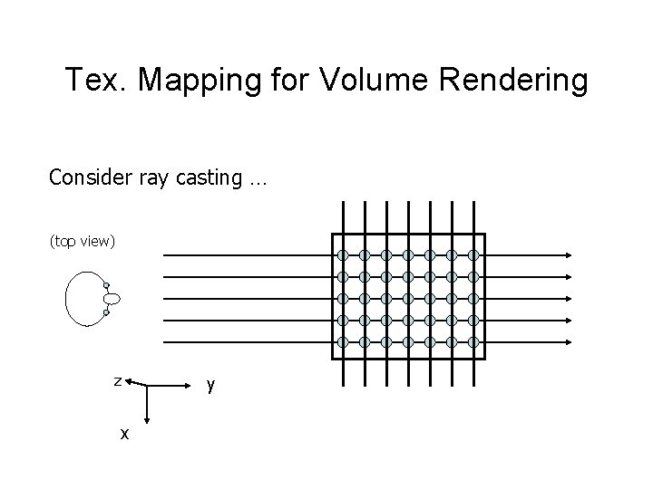
Tex. Mapping for Volume Rendering Consider ray casting … (top view) z x y

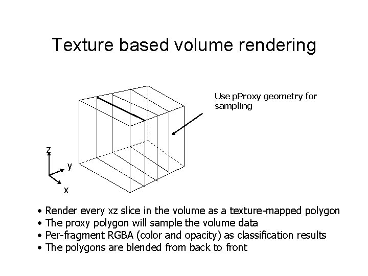
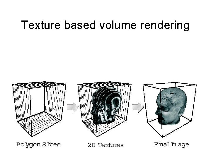
Texture based volume rendering Use p. Proxy geometry for sampling z y x • • Render every xz slice in the volume as a texture-mapped polygon The proxy polygon will sample the volume data Per-fragment RGBA (color and opacity) as classification results The polygons are blended from back to front

Texture based volume rendering

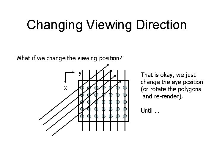
Changing Viewing Direction What if we change the viewing position? y x That is okay, we just change the eye position (or rotate the polygons and re-render), Until …

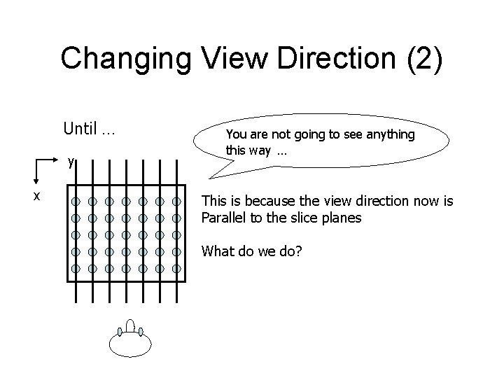
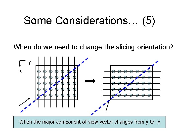
Changing View Direction (2) Until … y x You are not going to see anything this way … This is because the view direction now is Parallel to the slice planes What do we do?

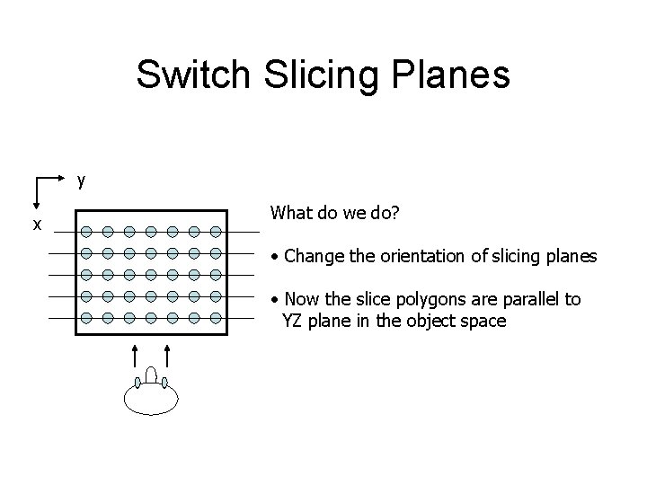
Switch Slicing Planes y x What do we do? • Change the orientation of slicing planes • Now the slice polygons are parallel to YZ plane in the object space

Some Considerations… (5) When do we need to change the slicing orientation? y x When the major component of view vector changes from y to -x

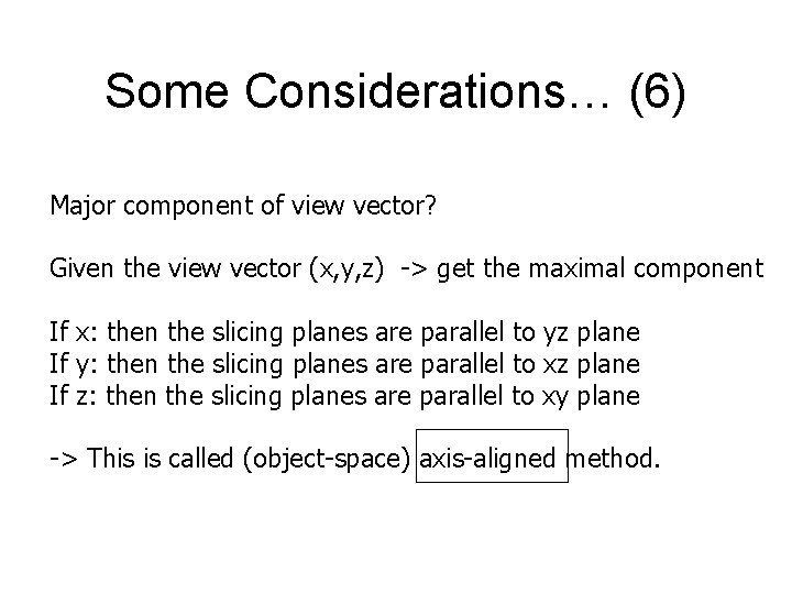
Some Considerations… (6) Major component of view vector? Given the view vector (x, y, z) -> get the maximal component If x: then the slicing planes are parallel to yz plane If y: then the slicing planes are parallel to xz plane If z: then the slicing planes are parallel to xy plane -> This is called (object-space) axis-aligned method.

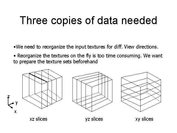
Three copies of data needed • We need to reorganize the input textures for diff. View directions. • Reorganize the textures on the fly is too time consuming. We want to prepare the texture sets beforehand z y x xz slices yz slices xy slices

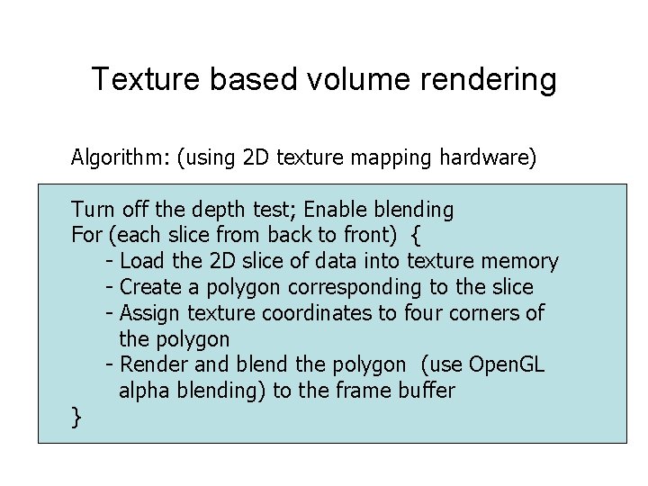
Texture based volume rendering Algorithm: (using 2 D texture mapping hardware) Turn off the depth test; Enable blending For (each slice from back to front) { - Load the 2 D slice of data into texture memory - Create a polygon corresponding to the slice - Assign texture coordinates to four corners of the polygon - Render and blend the polygon (use Open. GL alpha blending) to the frame buffer }

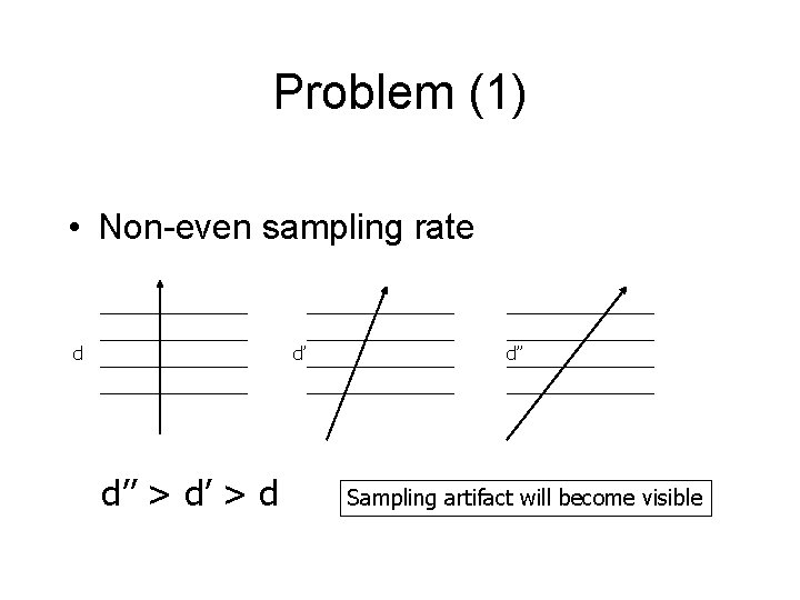
Problem (1) • Non-even sampling rate d d’ d’’ > d d’’ Sampling artifact will become visible

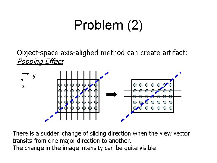
Problem (2) Object-space axis-alighed method can create artifact: Popping Effect y x There is a sudden change of slicing direction when the view vector transits from one major direction to another. The change in the image intensity can be quite visible

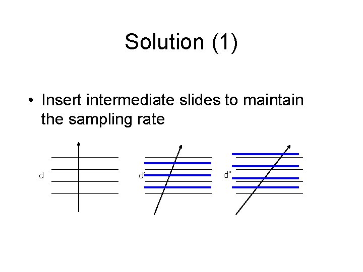
Solution (1) • Insert intermediate slides to maintain the sampling rate d d’ d’’

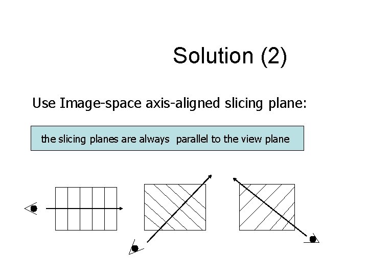
Solution (2) Use Image-space axis-aligned slicing plane: the slicing planes are always parallel to the view plane

3 D Texture Based Volume Rendering

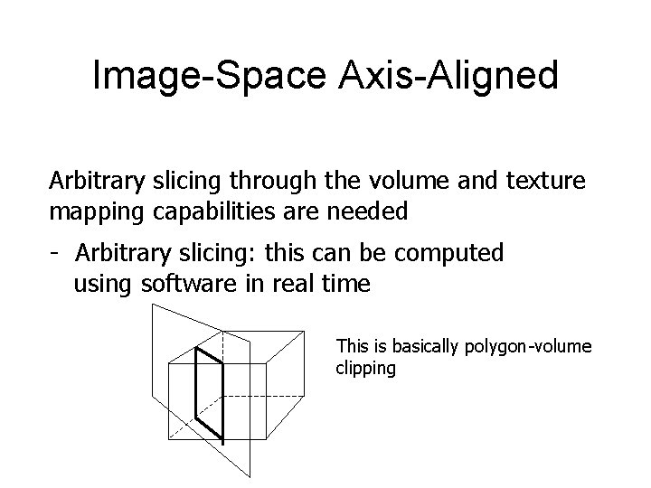
Image-Space Axis-Aligned Arbitrary slicing through the volume and texture mapping capabilities are needed - Arbitrary slicing: this can be computed using software in real time This is basically polygon-volume clipping

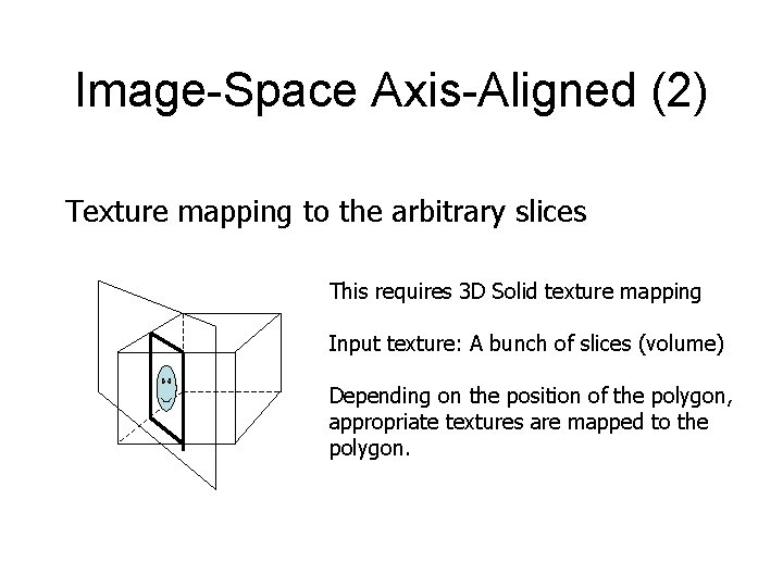
Image-Space Axis-Aligned (2) Texture mapping to the arbitrary slices This requires 3 D Solid texture mapping Input texture: A bunch of slices (volume) Depending on the position of the polygon, appropriate textures are mapped to the polygon.

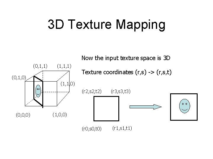
3 D Texture Mapping Now the input texture space is 3 D (0, 1, 1) (1, 1, 1) (0, 1, 0) Texture coordinates (r, s) -> (r, s, t) (1, 1, 0) (r 2, s 2, t 2) (0, 0, 0) (r 3, s 3, t 3) (1, 0, 0) (r 0, s 0, t 0) (r 1, s 1, t 1)

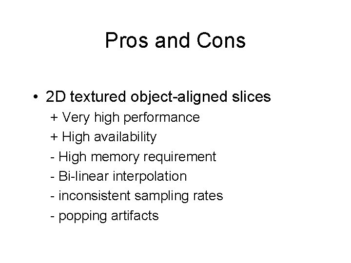
Pros and Cons • 2 D textured object-aligned slices + Very high performance + High availability - High memory requirement - Bi-linear interpolation - inconsistent sampling rates - popping artifacts

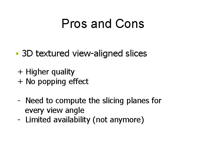
Pros and Cons § 3 D textured view-aligned slices + Higher quality + No popping effect - Need to compute the slicing planes for every view angle - Limited availability (not anymore)

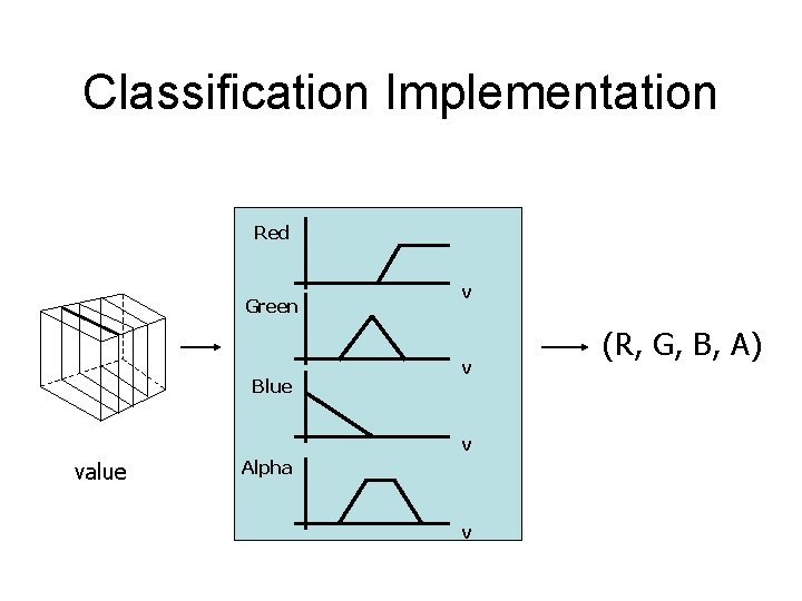
Classification Implementation Red Green Blue v value Alpha v (R, G, B, A)

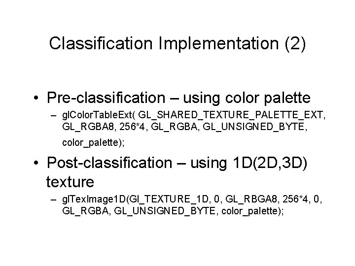
Classification Implementation (2) • Pre-classification – using color palette – gl. Color. Table. Ext( GL_SHARED_TEXTURE_PALETTE_EXT, GL_RGBA 8, 256*4, GL_RGBA, GL_UNSIGNED_BYTE, color_palette); • Post-classification – using 1 D(2 D, 3 D) texture – gl. Tex. Image 1 D(Gl_TEXTURE_1 D, 0, GL_RBGA 8, 256*4, 0, GL_RGBA, GL_UNSIGNED_BYTE, color_palette);

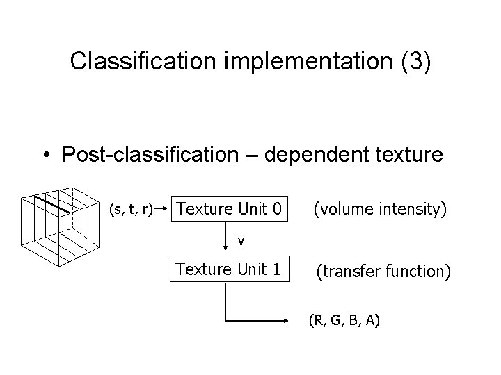
Classification implementation (3) • Post-classification – dependent texture (s, t, r) Texture Unit 0 (volume intensity) v Texture Unit 1 (transfer function) (R, G, B, A)

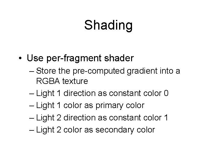
Shading • Use per-fragment shader – Store the pre-computed gradient into a RGBA texture – Light 1 direction as constant color 0 – Light 1 color as primary color – Light 2 direction as constant color 1 – Light 2 color as secondary color

Non-polygonal isosurface • Store voxel gradient as GRB texture • Store the volume density as alpha • Use Open. GL alpha test to discard volume density not equal to the threshold • Use the gradient texture to perform shading

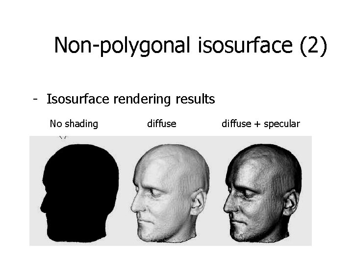
Non-polygonal isosurface (2) - Isosurface rendering results No shading diffuse + specular