Direct Vlasov solvers part I Nicolas Mounet CERNBEABPHSC

Direct Vlasov solvers – part I Nicolas Mounet, CERN/BE-ABP-HSC Acknowledgements: Xavier Buffat, Giovanni Iadarola, Kevin Li, Elias Métral, Adrian Oeftiger, Giovanni Rumolo

Direct Vlasov solvers Part I Ø Introduction: collective effects Ø Motivation for Vlasov solvers Ø Vlasov equation, in plasma physics and in the context of accelerators Ø Building of a simple Vlasov solver for impedance instabilities Part II Ø Alternative, compact way to present theory: Hamiltonians, Poisson’s brackets Ø Extensions: chromaticity, headtail modes, Landau damping, damper Ø Convergence issues Ø Benchmarks (HEADTAIL vs. MOSES) Ø Some results of various Vlasov solvers N. MOUNET – VLASOV SOLVERS I – CAS 21/11/2018 2

Collective effects Ø Collective effects: phenomena in which the evolution of the particle beam cannot be studied as if the beam was a collection of single particles behaving independently, but rather as an ensemble of interacting particles. Ø Examples (with the potential effect on the beam): ü Impedance & wake fields, i. e. interaction with the beam’s own selfgenerated electromagnetic (EM) fields (instabilities, heat load), ü Intra-beam scattering & Touschek effect (emittance growth, intensity loss), ü Interactions with trapped ions (coherent instabilities), ü Build up of an electron cloud and interaction with it (heat load, coherent instabilities), ü Interaction with another counter-rotating beam – so-called beam effects (emittance growth, intensity loss, possibly coherent instabilities). N. MOUNET – VLASOV SOLVERS I – CAS 21/11/2018 3

Collective effects - modeling instabilities Ø Coherent instability: self-enhanced, exponentially growing, oscillation of the full beam (or a significant part of it, e. g. one bunch). Ø A first approach is simply to perform multi-particle tracking (see previous CAS lectures), including the collective effect under study (e. g. collision between particles, EM fields from ensemble of particles, etc. ). Ø This approach is, in principle: ü simple and efficient, especially if a model is available for the self-interaction fields (e. g. wake function, frozen space charge, etc. ), ü easy to extend to complex situations, ü potentially very realistic. So why should we do anything else than this? N. MOUNET – VLASOV SOLVERS I – CAS 21/11/2018 4

Motivation for another kind of modeling Ø Multi-particle tracking still exhibit a number of drawbacks: ✗ It can be slow: one needs to track thousands to millions of macroparticles, sometimes with a complex interaction mechanism (PIC solver, bunch slicing for wake fields, etc. ). ✗ Most importantly, it does not always help for an understanding of what’s happening. ⇒ It’s not always easy to understand what parameters are the important ones to e. g. stabilize an unstable beam. N. MOUNET – VLASOV SOLVERS I – CAS 21/11/2018 5

Motivation for another kind of modeling Ø Multi-particle tracking can also be misleading: as a time domain technique, a beam that looks stable might actually be unstable if we track more turns. Example: average vertical position in the LHC vs octupole current Ioct (i. e. with increasing damping from transverse non-linearities): If we stop the simulation here, Ioct≥ 110 A is stable If we stop the simulation here, Ioct ≥ 100 A is stable N. MOUNET – VLASOV SOLVERS I – CAS 21/11/2018 If we stop the simulation here, Ioct≥ 120 A is stable What is the real threshold? Are we really stable for Ioct≥ 140 A? 6

Alternative for instability computation Ø Multi-particles is one way to discretize the phase space – very close to reality as the beams are indeed made of distinct particles, albeit much more numerous than in typical simulations. Ø A contrario, one can also consider the whole phase space distribution as a continuum, and look for modes arising from collective interactions, that could develop and lead to instabilities. ⇒ Vlasov solvers – named after the equation to be solved. ⇒ Switch from time to mode domain, the stability of each mode being predictable irrespectively of its rapidity to develop. Ø Historically, this was the first approach adopted to try to understand instabilities in particle accelerators [L. J. Laslett, V. K. Neil, and A. M. Sessler (1965), F. J. Sacherer (1972)]. N. MOUNET – VLASOV SOLVERS I – CAS 21/11/2018 7

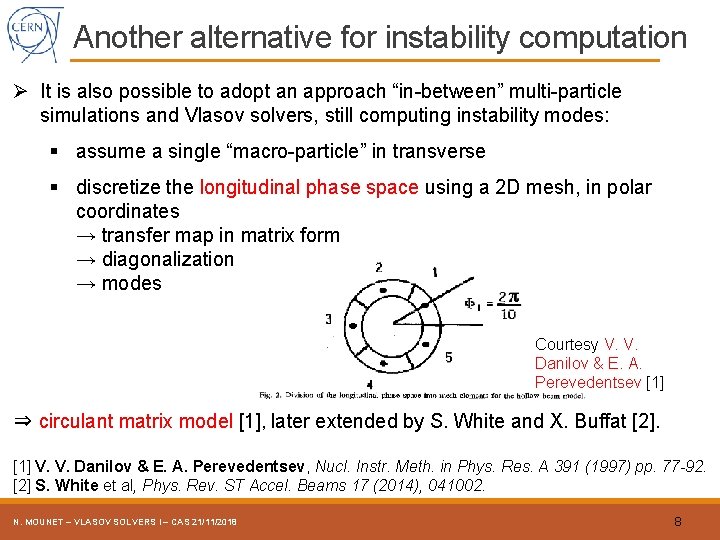
Another alternative for instability computation Ø It is also possible to adopt an approach “in-between” multi-particle simulations and Vlasov solvers, still computing instability modes: § assume a single “macro-particle” in transverse § discretize the longitudinal phase space using a 2 D mesh, in polar coordinates → transfer map in matrix form → diagonalization → modes Courtesy V. V. Danilov & E. A. Perevedentsev [1] ⇒ circulant matrix model [1], later extended by S. White and X. Buffat [2]. [1] V. V. Danilov & E. A. Perevedentsev, Nucl. Instr. Meth. in Phys. Res. A 391 (1997) pp. 77 -92. [2] S. White et al, Phys. Rev. ST Accel. Beams 17 (2014), 041002. N. MOUNET – VLASOV SOLVERS I – CAS 21/11/2018 8

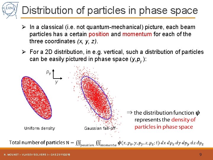
Distribution of particles in phase space Ø In a classical (i. e. not quantum-mechanical) picture, each beam particles has a certain position and momentum for each of the three coordinates (x, y, z). Ø For a 2 D distribution, in e. g. vertical, such a distribution of particles can be easily pictured in phase space (y, py ): py y N. MOUNET – VLASOV SOLVERS I – CAS 21/11/2018 9

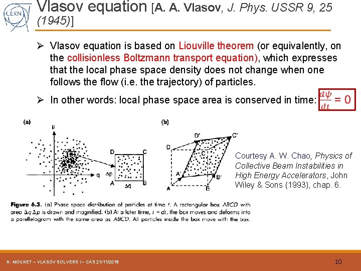
Vlasov equation [A. A. Vlasov, J. Phys. USSR 9, 25 (1945)] Ø Vlasov equation is based on Liouville theorem (or equivalently, on the collisionless Boltzmann transport equation), which expresses that the local phase space density does not change when one follows the flow (i. e. the trajectory) of particles. Ø In other words: local phase space area is conserved in time: Courtesy A. W. Chao, Physics of Collective Beam Instabilities in High Energy Accelerators, John Wiley & Sons (1993), chap. 6. N. MOUNET – VLASOV SOLVERS I – CAS 21/11/2018 10

Vlasov equation Ø Vlasov equation was first written in the context of plasma physics, where the standard collision-based Boltzmann approach, with Coulomb collisions, was failing. Ø As Coulomb interactions have a long-range character, the idea of Vlasov was to integrate the collective, self-interaction EM fields into the Hamiltonian, instead of writing them as collision term. Ø Assumptions: § conservative & deterministic system (governed by Hamiltonian) – no damping or diffusion from external sources (no synchrotron radiation), § particles are interacting only through the collective EM fields (no short-range collision). N. MOUNET – VLASOV SOLVERS I – CAS 21/11/2018 11

Vlasov solvers for synchrotrons Ø Vlasov solvers can be used in principle for various kinds of collective effects involving self-generated EM fields, e. g. : § Beam-beam effects [Y. Alexahin, Nucl. Instr. Meth. in Phys. Res. A 480 (2002) pp. 253– 288], § Electron-cloud, or more generally two stream effects [R. C. Davidson, Phys. Lett. A, 252 5 (1999) pp. 213 -221], § Space-charge & Impedance [M. Blaskiewicz, Phys. Rev. ST Accel. Beams 1 (1998), 044201]. Ø In this lecture we will rather focus on impedance effects without space-charge, in circular machines, i. e. the effects of the EM fields generated by a single-beam on itself through its interaction with the beam surroundings (vacuum pipe, cavities, collimators, etc. ). N. MOUNET – VLASOV SOLVERS I – CAS 21/11/2018 12

Vlasov solvers for impedance: brief review Ø Vlasov equation was first used to compute stability conditions for a given excitation, obtaining dispersion relations, by Laslett et al (1965) [1]. Ø The seminal Sacherer integral equation was derived (1972) [2], and a simple formula for instability growth rates obtained from it (1974) [3]. Ø Besnier devised a method to solve Sacherer Integral eq. using orthogonal polynomials (1979) [4], and Laclare developped an equivalent approach in frequency domain (1985) [5]. Ø Several codes were implemented over the years, e. g. MOSES (1985) [6], NHTVS (2014) [7], DELPHI [8] (2014) and GALACTIC (2018) [9]. Ø Extension to include synchrotron radiation for lepton machines do exist, solving Vlasov. Fokker-Planck equation, see e. g. Ref. [10]. Ø Reviews, courses and books can be found, in e. g. Refs. [3, 5] and Chao’s book [11]. [1] L. J. Laslett, V. K. Neil, and A. M. Sessler, Rev. Sci. Instrum. 36, 4 (1965) pp. 436– 448. [2] F. J. Sacherer, CERN/SI-BR/72 -5 (1972). [3] B. Zotter & F. J. Sacherer, Proc. 1 st Int. School Part. Acc. , Erice, Italy (1976) pp. 175– 218. [4] G. Besnier, D. Brandt, and B. Zotter, CERN LEP- TH/84 -11, LHC Note 17 (1985). [5] J. L. Laclare, Proc. CERN Accelerator School, Oxford, UK (1985) pp. 264– 326. N. MOUNET – VLASOV SOLVERS I – CAS 21/11/2018 [6] Y. -H. Chin, CERN/SPS/85 -2 (1985) and CERN/LEP-TH/88 -05 (1988). [7] A. V. Burov, Phys. Rev. ST Accel. Beams, 17 (2014) 021007. [8] N. Mounet, CERN Yellow Reports: Conference Proceedings, 1 (2018) p. 77. [9] E. Me tral et al, Proc. IPAC’ 18, Vancouver, Canada (2018) pp. 3076– 3079. [10] R. L. Warnock, Nucl. Instr. Meth. in Phys. Res. A 561 (2006) pp. 186– 194. [11] A. W. Chao, Physics of Collective Beams Instabilities in High Energy Accelerators. John Wiley and Sons (1993), chap. 6. 13

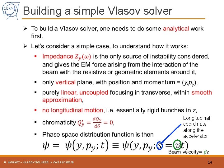
Building a simple Vlasov solver Longitudinal coordinate along the accelerator N. MOUNET – VLASOV SOLVERS I – CAS 21/11/2018 14

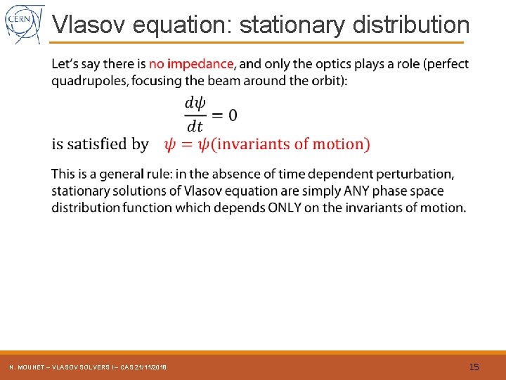
Vlasov equation: stationary distribution N. MOUNET – VLASOV SOLVERS I – CAS 21/11/2018 15

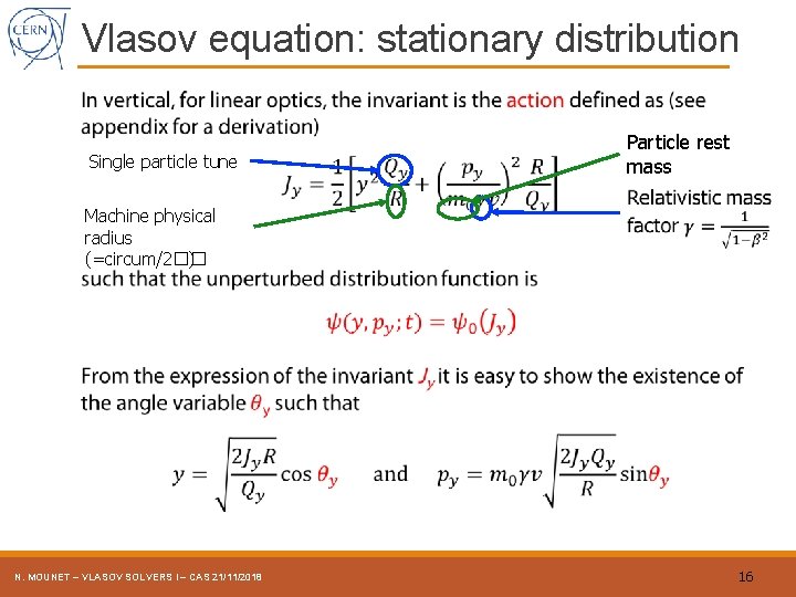
Vlasov equation: stationary distribution Single particle tune Machine physical radius (=circum/2�� ) N. MOUNET – VLASOV SOLVERS I – CAS 21/11/2018 Particle rest mass 16

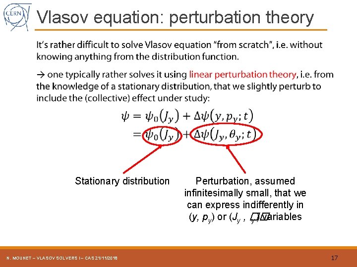
Vlasov equation: perturbation theory Stationary distribution N. MOUNET – VLASOV SOLVERS I – CAS 21/11/2018 Perturbation, assumed infinitesimally small, that we can express indifferently in (y, py) or (Jy , �� y ) variables 17

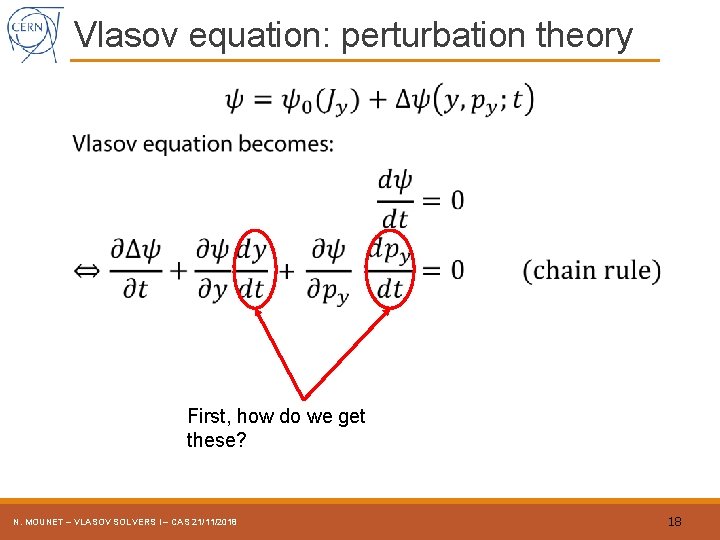
Vlasov equation: perturbation theory First, how do we get these? N. MOUNET – VLASOV SOLVERS I – CAS 21/11/2018 18

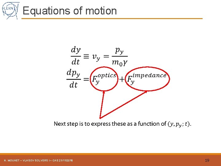
Equations of motion N. MOUNET – VLASOV SOLVERS I – CAS 21/11/2018 19

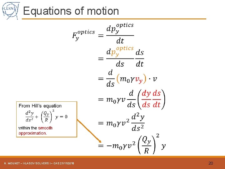
Equations of motion N. MOUNET – VLASOV SOLVERS I – CAS 21/11/2018 20

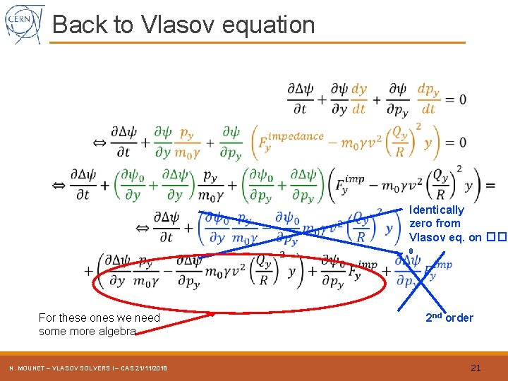
Back to Vlasov equation Identically zero from Vlasov eq. on �� 0 For these ones we need some more algebra N. MOUNET – VLASOV SOLVERS I – CAS 21/11/2018 2 nd order 21

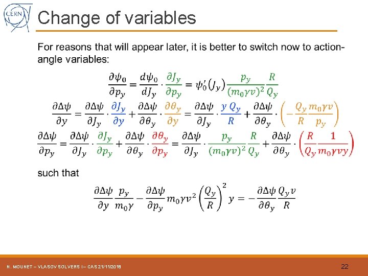
Change of variables N. MOUNET – VLASOV SOLVERS I – CAS 21/11/2018 22

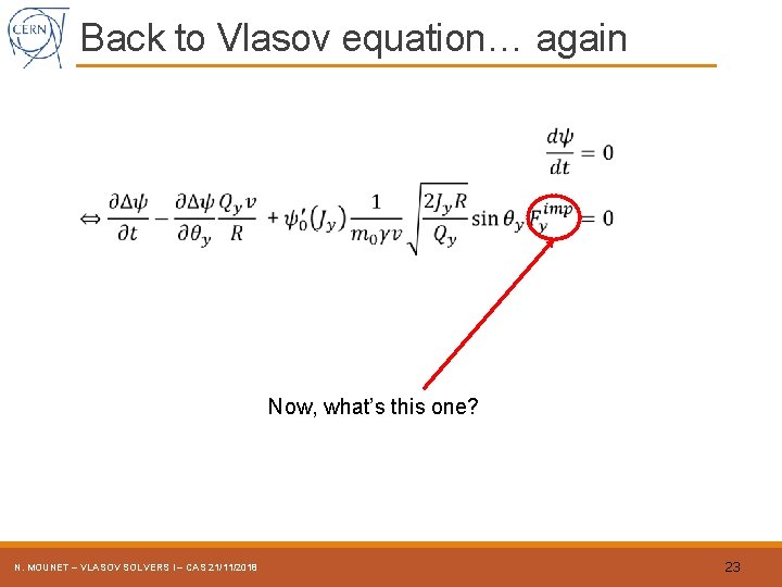
Back to Vlasov equation… again Now, what’s this one? N. MOUNET – VLASOV SOLVERS I – CAS 21/11/2018 23

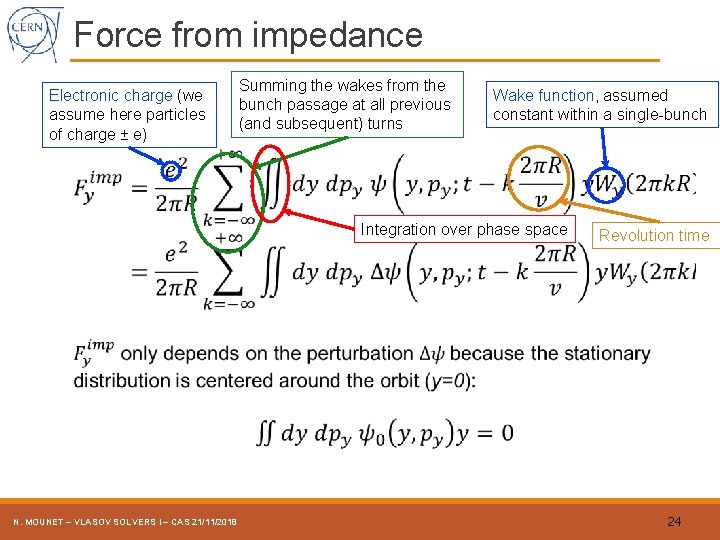
Force from impedance Electronic charge (we assume here particles of charge ± e) Summing the wakes from the bunch passage at all previous (and subsequent) turns Wake function, assumed constant within a single-bunch Integration over phase space N. MOUNET – VLASOV SOLVERS I – CAS 21/11/2018 Revolution time 24

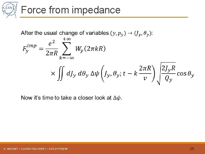
Force from impedance N. MOUNET – VLASOV SOLVERS I – CAS 21/11/2018 25

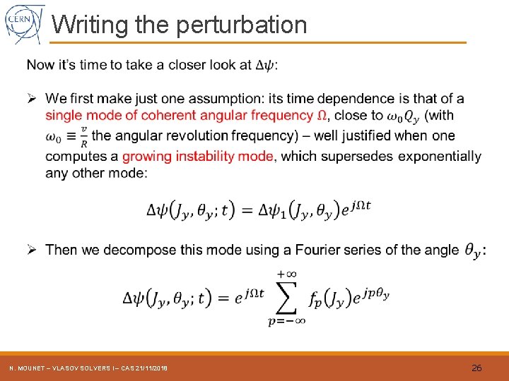
Writing the perturbation N. MOUNET – VLASOV SOLVERS I – CAS 21/11/2018 26

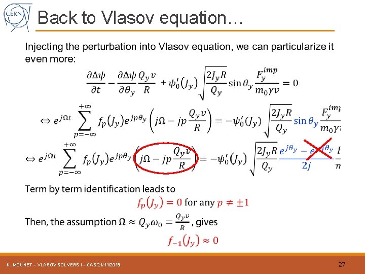
Back to Vlasov equation… N. MOUNET – VLASOV SOLVERS I – CAS 21/11/2018 27

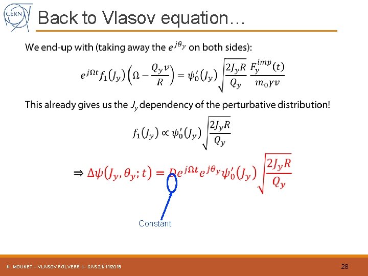
Back to Vlasov equation… Constant N. MOUNET – VLASOV SOLVERS I – CAS 21/11/2018 28

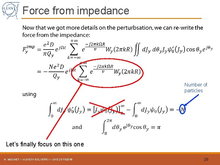
Force from impedance Number of particles Let’s finally focus on this one N. MOUNET – VLASOV SOLVERS I – CAS 21/11/2018 29

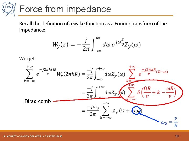
Force from impedance Dirac comb N. MOUNET – VLASOV SOLVERS I – CAS 21/11/2018 30

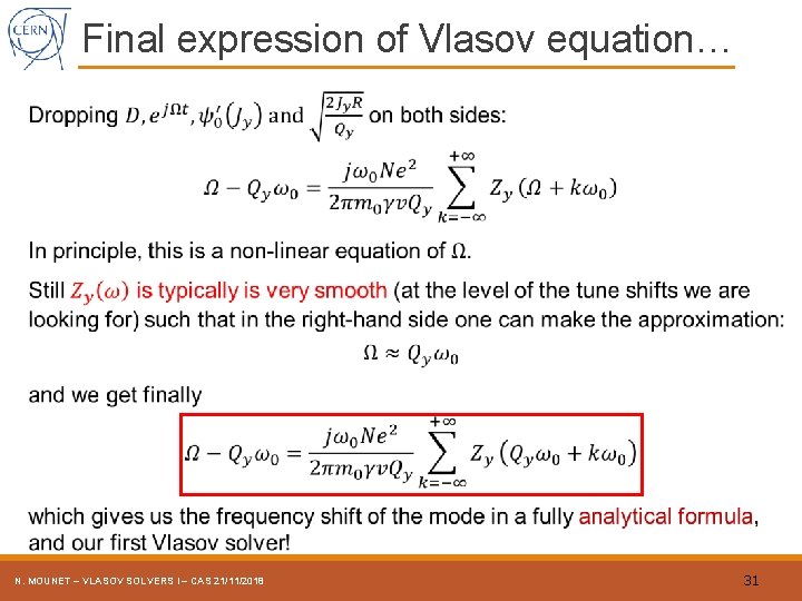
Final expression of Vlasov equation… N. MOUNET – VLASOV SOLVERS I – CAS 21/11/2018 31

Appendix N. MOUNET – VLASOV SOLVERS I – CAS 21/11/2018 32

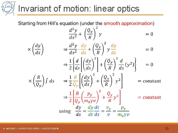
Invariant of motion: linear optics N. MOUNET – VLASOV SOLVERS I – CAS 21/11/2018 33

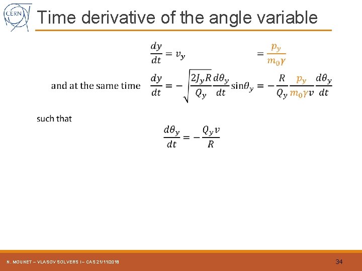
Time derivative of the angle variable N. MOUNET – VLASOV SOLVERS I – CAS 21/11/2018 34