Direct Method of Interpolation Industrial Engineering Majors Authors

Direct Method of Interpolation Industrial Engineering Majors Authors: Autar Kaw, Jai Paul http: //numericalmethods. eng. usf. edu Transforming Numerical Methods Education for STEM Undergraduates http: //numericalmethods. eng. usf. edu 1

Direct Method of Interpolation http: //numericalmethods. eng. usf. edu

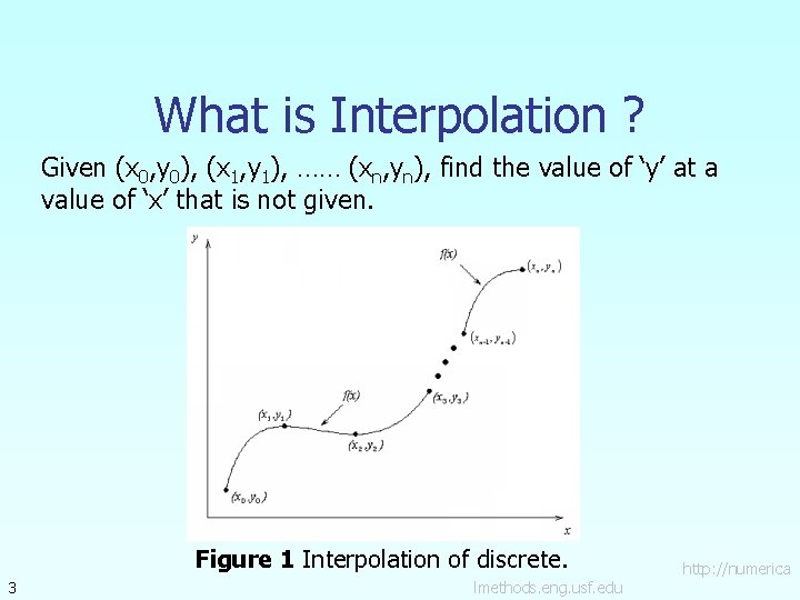
What is Interpolation ? Given (x 0, y 0), (x 1, y 1), …… (xn, yn), find the value of ‘y’ at a value of ‘x’ that is not given. Figure 1 Interpolation of discrete. 3 lmethods. eng. usf. edu http: //numerica

Interpolants Polynomials are the most common choice of interpolants because they are easy to: Evaluate Differentiate, and Integrate 4 lmethods. eng. usf. edu http: //numerica

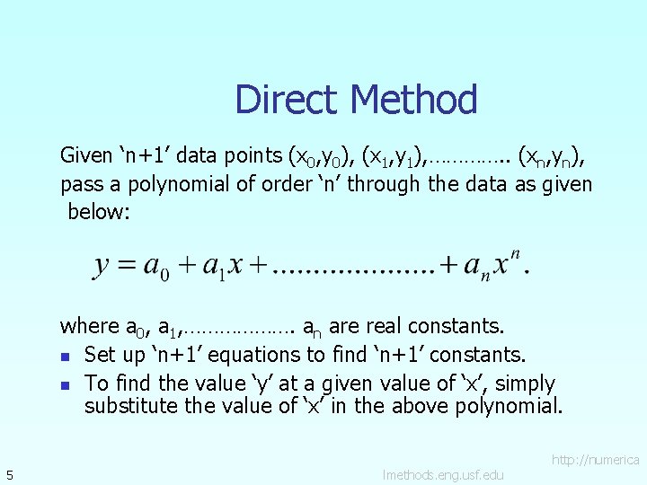
Direct Method Given ‘n+1’ data points (x 0, y 0), (x 1, y 1), …………. . (xn, yn), pass a polynomial of order ‘n’ through the data as given below: where a 0, a 1, ………………. an are real constants. n Set up ‘n+1’ equations to find ‘n+1’ constants. n To find the value ‘y’ at a given value of ‘x’, simply substitute the value of ‘x’ in the above polynomial. 5 lmethods. eng. usf. edu http: //numerica

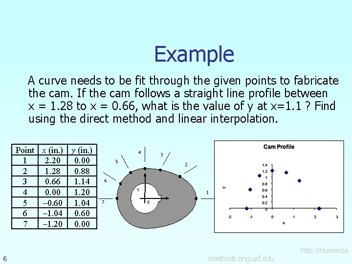
Example A curve needs to be fit through the given points to fabricate the cam. If the cam follows a straight line profile between x = 1. 28 to x = 0. 66, what is the value of y at x=1. 1 ? Find using the direct method and linear interpolation. Point 1 2 3 4 5 6 7 6 x (in. ) y (in. ) 2. 20 0. 00 1. 28 0. 88 0. 66 1. 14 0. 00 1. 20 – 0. 60 1. 04 – 1. 04 0. 60 – 1. 20 0. 00 4 3 5 2 6 Y 7 1 X lmethods. eng. usf. edu http: //numerica

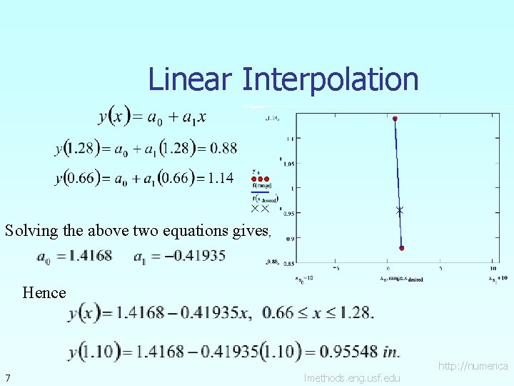
Linear Interpolation Solving the above two equations gives, Hence 7 lmethods. eng. usf. edu http: //numerica

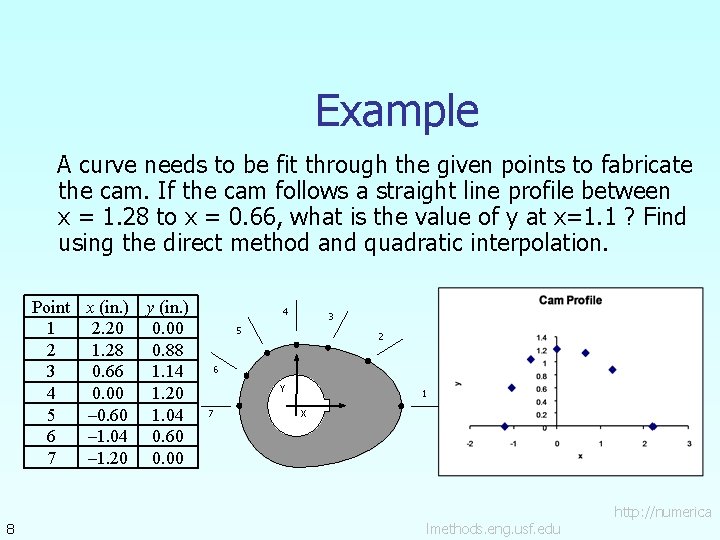
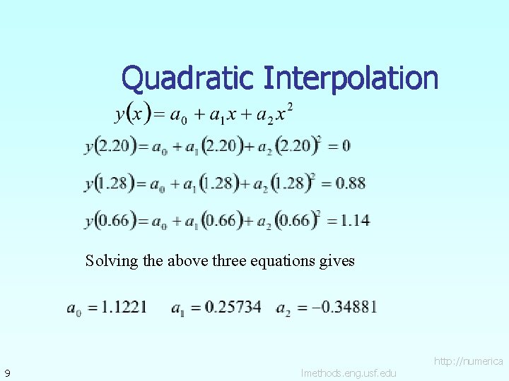
Example A curve needs to be fit through the given points to fabricate the cam. If the cam follows a straight line profile between x = 1. 28 to x = 0. 66, what is the value of y at x=1. 1 ? Find using the direct method and quadratic interpolation. Point 1 2 3 4 5 6 7 8 x (in. ) y (in. ) 2. 20 0. 00 1. 28 0. 88 0. 66 1. 14 0. 00 1. 20 – 0. 60 1. 04 – 1. 04 0. 60 – 1. 20 0. 00 4 3 5 2 6 Y 7 1 X lmethods. eng. usf. edu http: //numerica

Quadratic Interpolation Solving the above three equations gives 9 lmethods. eng. usf. edu http: //numerica

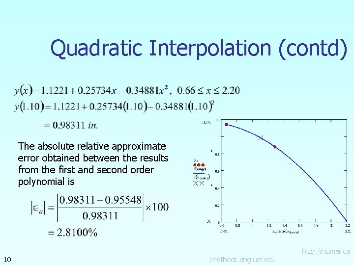
Quadratic Interpolation (contd) The absolute relative approximate error obtained between the results from the first and second order polynomial is 10 lmethods. eng. usf. edu http: //numerica

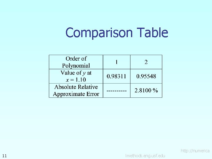
Comparison Table 11 lmethods. eng. usf. edu http: //numerica

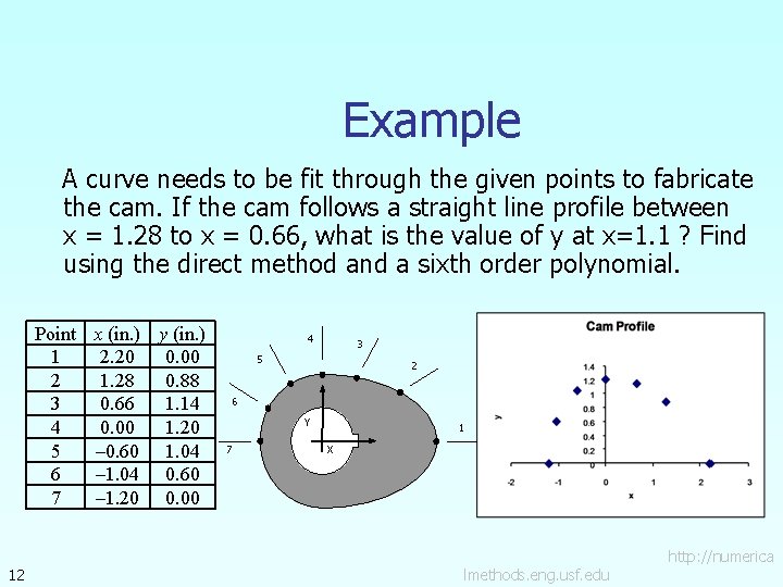
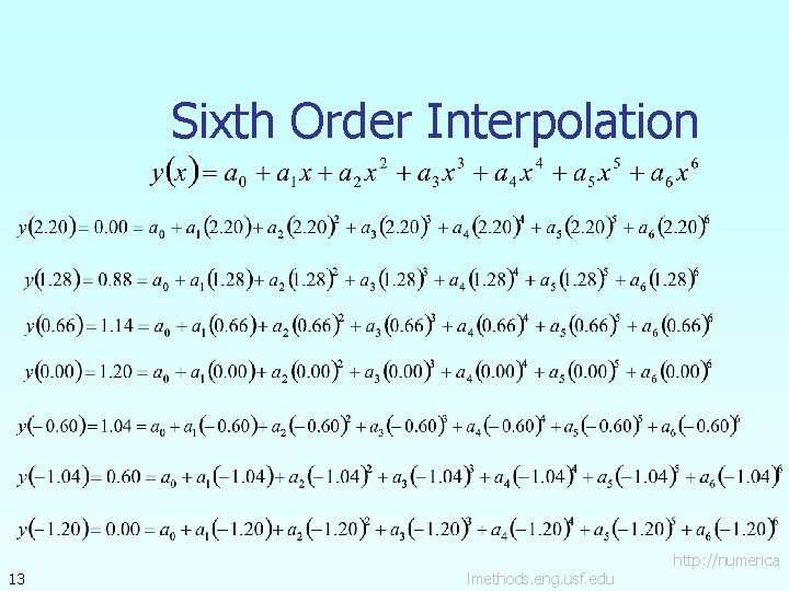
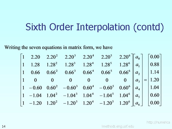
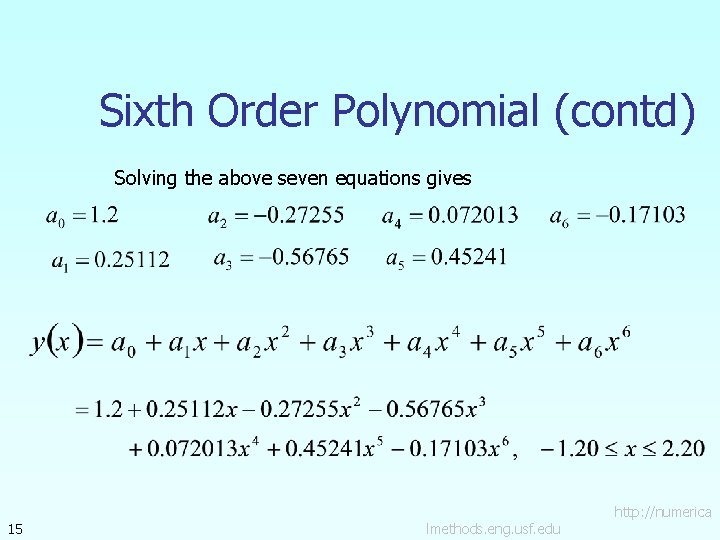
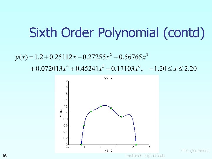
Example A curve needs to be fit through the given points to fabricate the cam. If the cam follows a straight line profile between x = 1. 28 to x = 0. 66, what is the value of y at x=1. 1 ? Find using the direct method and a sixth order polynomial. Point 1 2 3 4 5 6 7 12 x (in. ) y (in. ) 2. 20 0. 00 1. 28 0. 88 0. 66 1. 14 0. 00 1. 20 – 0. 60 1. 04 – 1. 04 0. 60 – 1. 20 0. 00 4 3 5 2 6 Y 7 1 X lmethods. eng. usf. edu http: //numerica

Sixth Order Interpolation 13 lmethods. eng. usf. edu http: //numerica

Sixth Order Interpolation (contd) 14 lmethods. eng. usf. edu http: //numerica

Sixth Order Polynomial (contd) Solving the above seven equations gives 15 lmethods. eng. usf. edu http: //numerica

Sixth Order Polynomial (contd) 16 lmethods. eng. usf. edu http: //numerica

Additional Resources For all resources on this topic such as digital audiovisual lectures, primers, textbook chapters, multiple-choice tests, worksheets in MATLAB, MATHEMATICA, Math. Cad and MAPLE, blogs, related physical problems, please visit http: //numericalmethods. eng. usf. edu/topics/direct_met hod. html

THE END http: //numericalmethods. eng. usf. edu