Direct Fit event reconstruction Method of the fit

Direct. Fit event reconstruction Method of the fit: exhaustive search • simulate cascade events with various x, y, z, q, j (and fit for E, t 0), and compare them to the data event. • optionally for each new track simulate cascades of equal energy spaced along the track and solve for best combination (next slide) • the simulated event that looks most like the data event is the result Advantages: • simple and robust • most precise description of ice can be used in reconstruction (SPICE Lea ice model: including tilt and anisotropy) Drawbacks: • can be very slow (~1 day/event) Dmitry Chirkin, UW Madison

Track reconstruction For each new track given by x, y, z, q, j, t 0, simulate cascades of equal energy at equal intervals along the track. Each cascade i creates hits in DOMs/time bins j: leaving charge Qij. For the pattern of hits that we actually have in data, qj, we can find the best representation of the event in terms of the simulated cascades by creating a weighted superposition (linear combination) of the cascades i. This can be done by maximizing the limited-simulation-statistics likelihood (LSSL) against the weights, starting with an NNLS solution to qj=wi. Qij. This is done for different t 0 and the t 0 maximizing the likelihood is chosen.

Comparing a simulation event with a data event Use the same likelihood function as in the SPICE Lea fit: includes Poisson fluctuations in data, simulation, and a 20% allowance for non-Poisson errors (in description of ice and others). All feature-extracted waveforms (charge histogram vs. time in a DOM) are binned in 25 ns bins, and then processed with a Bayesian blocks procedure, which combines low-count or nearly-same-charge bins. This is the same procedure as was used in the SPICE Lea fit. So, we are using exactly the same comparison procedure as was used in the ice model fit (here: SPICE Lea).

LSSL description Suppose we repeat the measurement in data nd times and in simulation ns times. The ms and md are the expectation mean values of counts per measurement in simulation and in data. With the total count in the combined set of simulation and data is s + d , the conditional probability distribution function of observing s simulation and d data counts is There is an obvious constraint which can be derived, e. g. , from the normalization condition

Two hypotheses: If data and simulation are unrelated and completely independent from each other, then we can maximize the likelihood for ms and md independently, which with the above constraint yields On the other hand, we can assume that data and simulation come from the same process, i. e. , We can compare the two hypotheses by forming a likelihood ratio

Example 2000 200 To enhance the differences between the two likelihood approaches, consider that the amount of simulation is only 1/10 th of that of data

Using full range of the data and simulation Simulated exp(-x/5. 0) with mean of 5. 0

Search algorithm 1. Start with x, y, z of COG, q=0, j=0, E=105 Ge. V, t 0=0 2. Propose 25 sets of cascade parameters x, y, z, q, j from a gaussian distribution with rms=10 m in x, y, z and rms=30 degrees in q, j. Keep the values of E and t 0. 3. For each proposed simulated event find the best E (by scaling the simulated event) and t 0 (by time-shifting the hits in the simulated event); calculate the likelihood L. 4. Out of these 25 event select the one with the best value of L and update the 7 cascade parameters; remember the best value of L: L*. 5. Repeat steps 2 -4 40 times. Use 20 events resulting from step 4 with the best values of L* to update the rms in x, y, z, and rms in q, j, and to establish correlation between these (important since the brightest point of the cascade is some distance away from the starting point along the cascade direction; also the Cherenkov light is emitted predominantly forward). 6. Repeat steps 2 -5 10 times; The final result is calculated by averaging simulated events with the best 160 values of L*. The rms of x, y, z, and the rms in q, j are also computed to provide a measure of uncertainties.

Other search algorithms and uncertainties The algorithm described on the previous slide is an optimized variant of • Localized random search. Other methods that I tried are: • Simultaneous perturbation stochastic approximation with and without the estimate of the second derivative (Newton-like method). • Markov chain with transitional probability defined by condition Li+1<Li. Although the rms values in cascade parameters obtained in the localized random search and Markov chain methods are probably related to the uncertainties of the measurement, the well-defined values of the uncertainties should probably be calculated by applying the reconstruction to a few (dozen? ) cascade events simulated with the same parameters.

Uncertainties with ABC (Approximate Bayesian Calculation) solves for an approximation to the posterior PDF when the likelihood function is not known or its calculation is intractable. We need a distance (in this case LSSL comparing simulation sets with data) and consider steps sampled from a proposal distribution which result in the distance smaller than a pre-set upper bound. All such steps are accepted. This is a reversible Markov Chain, with a stationary distribution being the posterior parameter PDF for events similar to the data event with LSSL<bound. This approximates the parameter PDF for the actual given data event. Statistical sampling is possible (performed for Bert). It is unclear if the systematical uncertainties can be included in this sampling procedure (due to curse of dimensionality).

Track reconstruction in 28 HE events Only 1 event out of 28 was reconstructed with the reconstructed track going through the hits left by the muon. In the other 6 events containing a track along with the interaction cascade the contribution to the likelihood from the smaller losses along the track are “washed out” by the fluctuations in the large contribution from the interaction cascade. this results in track missing the smaller hits left by the muon. possibly solved by over-simulating, however a factor x 10 did not help (although only tried on the first 3 muon events)

Loss pattern along track Dr. Strangepork Bert

llh vs. step number Dr. Strangepork Bert

z vs. llh Dr. Strangepork Bert

llh 1… 200 all 201… 400 Dr. Strangepork Bert

z 1… 200 all 201… 400 Dr. Strangepork Bert

t 0 vs. E Dr. Strangepork Bert

E 1… 200 all 201… 400 Dr. Strangepork Bert

t 0 1… 200 all 201… 400 Dr. Strangepork Bert

y vs. x Dr. Strangepork Bert

x 1… 200 all 201… 400 Dr. Strangepork Bert

y 1… 200 all 201… 400 Dr. Strangepork Bert

q vs. j Dr. Strangepork Bert

j 1… 200 all 201… 400 Dr. Strangepork Bert

q 1… 200 all 201… 400 Dr. Strangepork Bert

References Likelihood: • Likelihood description for comparing data with simulation (LSSL: limited simulation statistics likelihood), ar. Xiv: 1304. 0735 • Direct. Fit (and updated ice model): ar. Xiv: 1309. 7010 (ICRC, Rio) Direct. Fit experimental code: http: //icecube. wisc. edu/~dima/work/WISC/ppc/bkp/llh. tgz http: //code. icecube. wisc. edu/svn/projects/ppc/trunk/private/ppc/llh/

nvidia-smi -lsa GPU 0: Cudatest: lean and mean ice fitting machine Product Name Serial PCI ID Temperature : Ge. Force GTX 295 : 1803836293359 : 5 eb 10 de : 87 C GPU 1: cudatest: Product Name : Ge. Force GTX 295 Serial : 2497590956570 Found 6 devices, PCI IDdriver 2030, runtime 2030 : 5 eb 10 de Temperature : 90 C 0(1. 3): Ge. Force GTX 295 1. 296 GHz G(939261952) S(16384) C(65536) R(16384) W(32) GPU 2: l 1 o 1 c 0 h 1 i 0 m 30 a 256 M(262144) T(512: 512, 64) G(65535, 1) Product Name : Ge. Force GTX 295 1(1. 3): Ge. Force GTX 295 1. 296 GHz G(939261952) S(16384) C(65536) R(16384) W(32) Serial : 1247671583504 l 0 PCI o 1 ID c 0 h 1 i 0 m 30 a 256 M(262144) : T(512: 512, 64) G(65535, 1) 5 eb 10 de 2(1. 3): Ge. Force GTX 295 1. 296 GHz G(939261952) S(16384) C(65536) R(16384) W(32) Temperature : 100 C l 0 o 1 c 0 h 1 i 0 m 30 a 256 M(262144) T(512: 512, 64) G(65535, 1) GPU 3: Product Name : Ge. Force GTX 295 3(1. 3): Ge. Force GTX 295 1. 296 GHz G(938803200) S(16384) C(65536) R(16384) W(32) Serial : 2353575330598 l 0 o 1 c 0 h 1 i 0 m 30 a 256 M(262144) T(512: 512, 64) G(65535, 1) PCI ID : 5 eb 10 de 4(1. 3): Ge. Force GTX 295 1. 296 GHz G(939261952) S(16384) C(65536) R(16384) W(32) Temperature : 105 C l 0 o 1 c 0 h 1 i 0 m 30 a 256 M(262144) T(512: 512, 64) G(65535, 1) GPU 4: 5(1. 3): Ge. Force GTX 295 1. 296 GHz G(939261952) S(16384) C(65536) R(16384) W(32) Product Name : Ge. Force GTX 295 l 0 Serial o 1 c 0 h 1 i 0 m 30 a 256 M(262144) : T(512: 512, 64) G(65535, 1) 1939228426794 PCI ID : 5 eb 10 de Temperature : 100 C GPU 5: Product Name : Ge. Force GTX 295 Serial : 2347233542940 PCI ID : 5 eb 10 de 3 GTX 295 cards, each with 2 GPUs Temperature : 103 C As fast as 900 CPU cores 2 and 3 4 and 5 0 and 1 PSU

GZK 9000 GPU Cluster Deployed in 2012 at the WID/MIR datacenter (shared with CHTC @ 30%) 12 servers, each with 2 x AMD 6176 ( 12 cores/CPU) 4 x GPUs Nvidia Tesla M 2070 (448 CUDA cores/GPU)

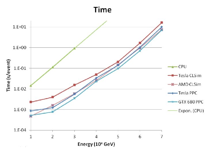
Performance vs. Price

Production optimizations