Direct and iterative sparse linear solvers applied to

Direct and iterative sparse linear solvers applied to groundwater flow simulations Matrix Analysis and Applications October 2007

Jocelyne Erhel INRIA Rennes Jean-Raynald de Dreuzy CNRS, Geosciences Rennes Anthony Beaudoin LMPG, Le Havre Partly funded by Grid’ 5000 french project

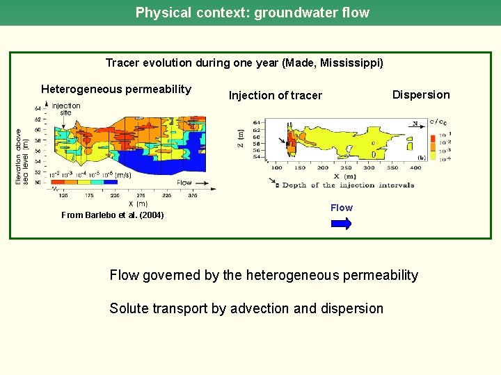
Physical context: groundwater flow Tracer evolution during one year (Made, Mississippi) Heterogeneous permeability From Barlebo et al. (2004) Dispersion Injection of tracer Flow governed by the heterogeneous permeability Solute transport by advection and dispersion

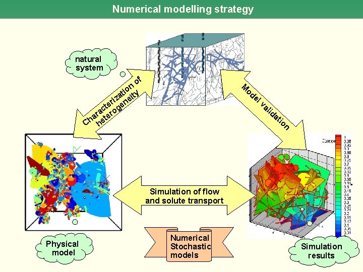
Numerical modelling strategy natural system of n io ty t iza nei r te ge c ra ero a t Ch he M od el va lid at io n Head Simulation of flow and solute transport Physical model Numerical Stochastic models Simulation results

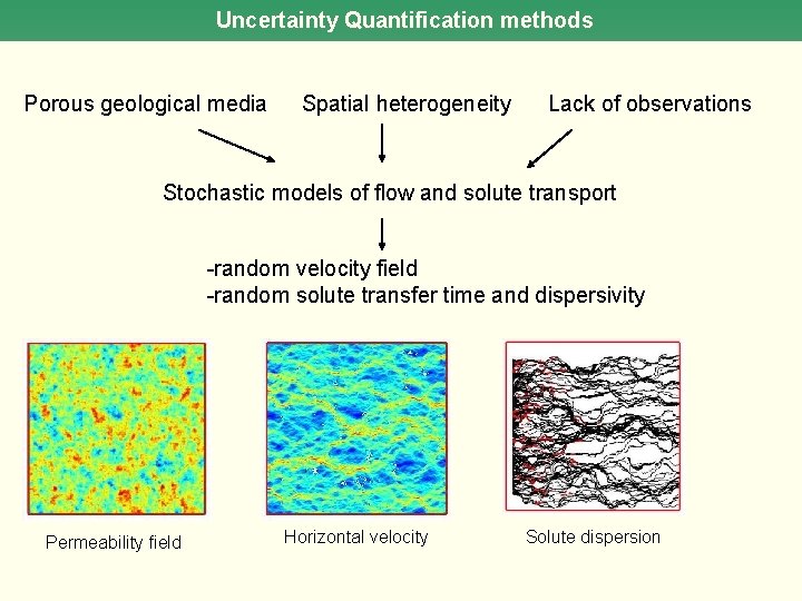
Uncertainty Quantification methods Porous geological media Spatial heterogeneity Lack of observations Stochastic models of flow and solute transport -random velocity field -random solute transfer time and dispersivity Permeability field Horizontal velocity Solute dispersion

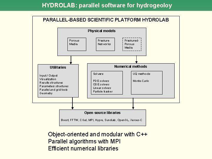
HYDROLAB: parallel software for hydrogeoloy PARALLEL-BASED SCIENTIFIC PLATFORM HYDROLAB Physical models Porous Media Fracture Networks Numerical methods Utilitaries Input / Output Visualization Results structures Parameters structures Parallel and grid tools Geometry Fractured. Porous Media Solvers UQ methods PDE solvers ODE solvers Linear solvers Particle tracker Monte-Carlo Open source libraries Boost, FFTW, CGal, MPI, Hypre, Sundials, Open. GL, Xerces-C Object-oriented and modular with C++ Parallel algorithms with MPI Efficient numerical libraries

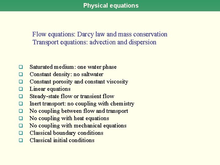
Physical equations Flow equations: Darcy law and mass conservation Transport equations: advection and dispersion q q q Saturated medium: one water phase Constant density: no saltwater Constant porosity and constant viscosity Linear equations Steady-state flow or transient flow Inert transport: no coupling with chemistry No coupling between flow and transport No coupling with heat equations No coupling with mechanical equations Classical boundary conditions Classical initial conditions

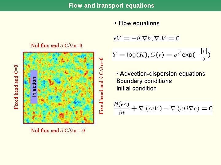
Flow and transport equations • Flow equations Nul flux and C/ n = 0 Fixed head and C/ n=0 injection Fixed head and C=0 Nul flux and C/ n=0 • Advection-dispersion equations Boundary conditions Initial condition

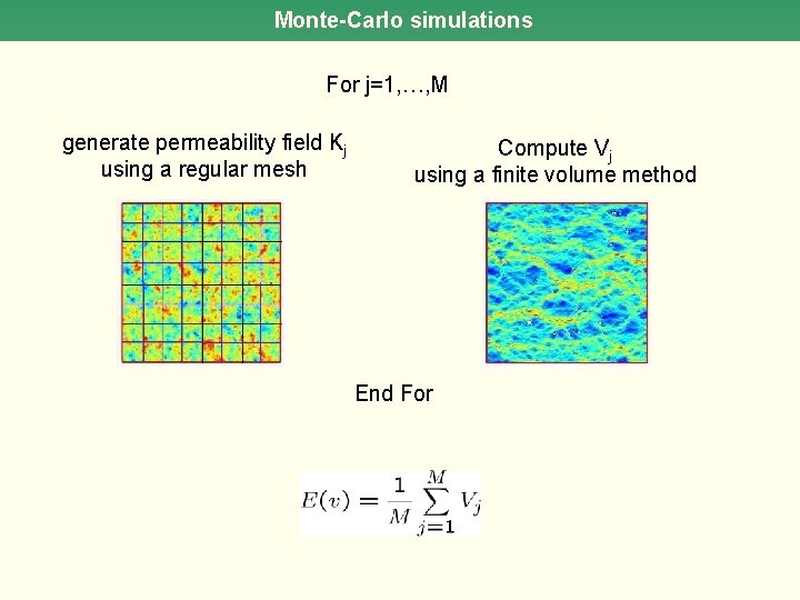
Monte-Carlo simulations For j=1, …, M generate permeability field Kj using a regular mesh Compute Vj using a finite volume method End For

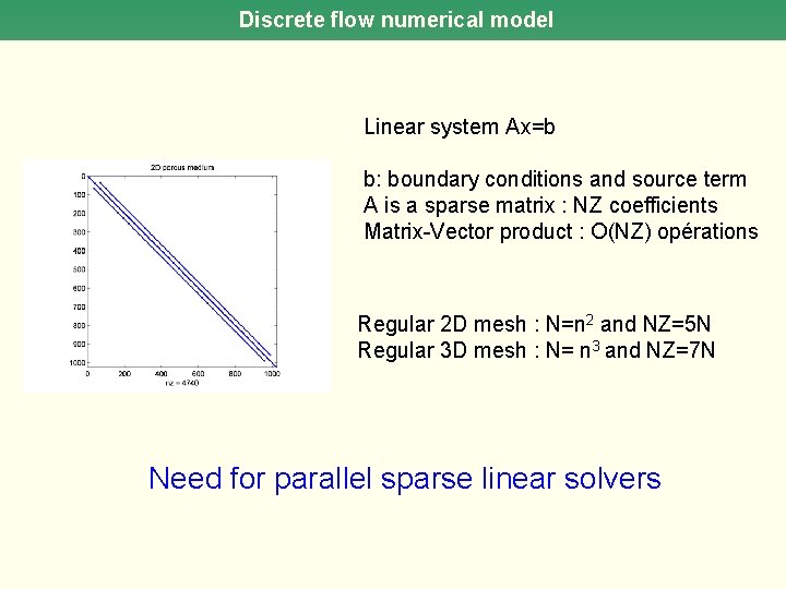
Discrete flow numerical model Linear system Ax=b b: boundary conditions and source term A is a sparse matrix : NZ coefficients Matrix-Vector product : O(NZ) opérations Regular 2 D mesh : N=n 2 and NZ=5 N Regular 3 D mesh : N= n 3 and NZ=7 N Need for parallel sparse linear solvers

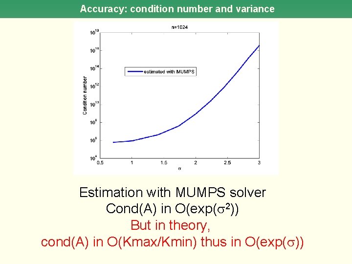
Accuracy: condition number and variance Estimation with MUMPS solver Cond(A) in O(exp( 2)) But in theory, cond(A) in O(Kmax/Kmin) thus in O(exp( ))

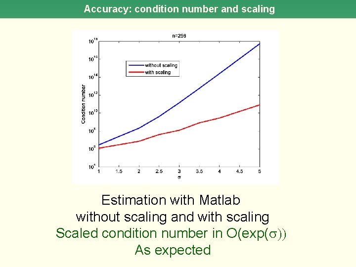
Accuracy: condition number and scaling Estimation with Matlab without scaling and with scaling Scaled condition number in O(exp( )) As expected

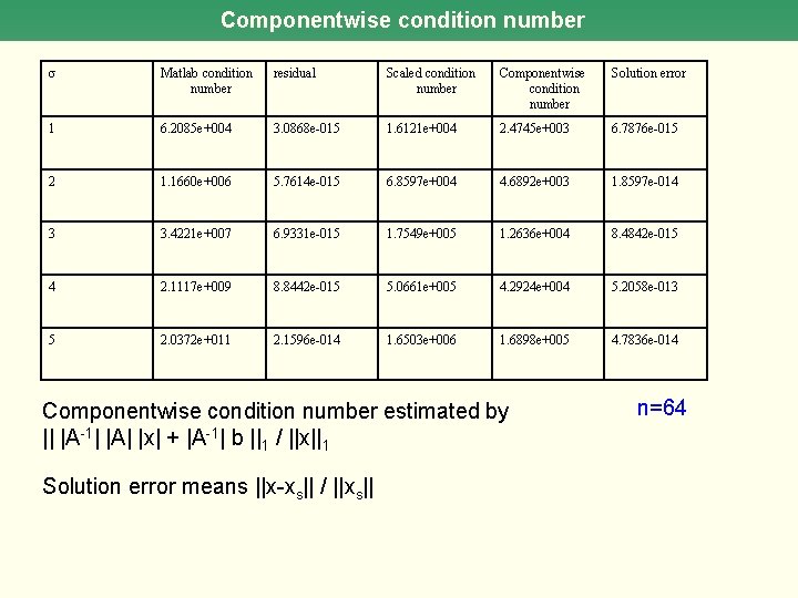
Componentwise condition number Matlab condition number residual Scaled condition number Componentwise condition number Solution error 1 6. 2085 e+004 3. 0868 e-015 1. 6121 e+004 2. 4745 e+003 6. 7876 e-015 2 1. 1660 e+006 5. 7614 e-015 6. 8597 e+004 4. 6892 e+003 1. 8597 e-014 3 3. 4221 e+007 6. 9331 e-015 1. 7549 e+005 1. 2636 e+004 8. 4842 e-015 4 2. 1117 e+009 8. 8442 e-015 5. 0661 e+005 4. 2924 e+004 5. 2058 e-013 5 2. 0372 e+011 2. 1596 e-014 1. 6503 e+006 1. 6898 e+005 4. 7836 e-014 Componentwise condition number estimated by || |A-1| |A| |x| + |A-1| b ||1 / ||x||1 Solution error means ||x-xs|| / ||xs|| n=64

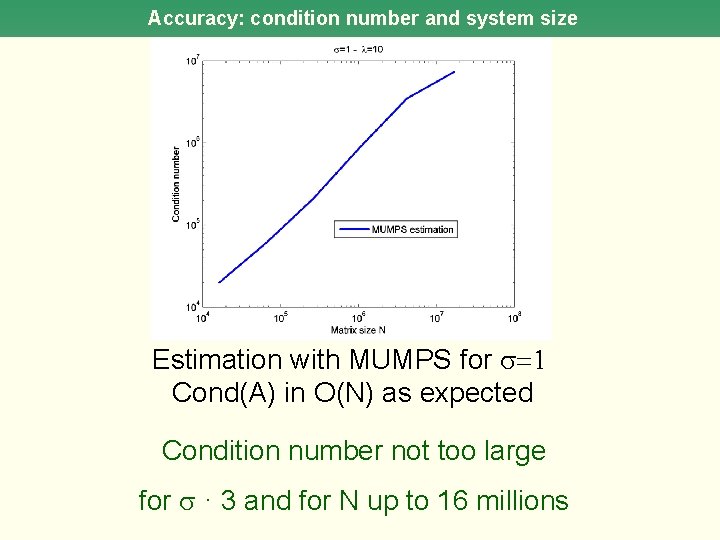
Accuracy: condition number and system size Estimation with MUMPS for =1 Cond(A) in O(N) as expected Condition number not too large for · 3 and for N up to 16 millions

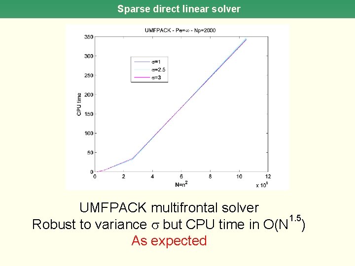
Sparse direct linear solver UMFPACK multifrontal solver 1. 5 Robust to variance but CPU time in O(N ) As expected

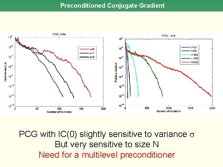
Preconditioned Conjugate Gradient PCG with IC(0) slightly sensitive to variance But very sensitive to size N Need for a multilevel preconditioner

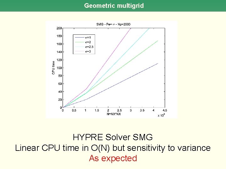
Geometric multigrid HYPRE Solver SMG Linear CPU time in O(N) but sensitivity to variance As expected

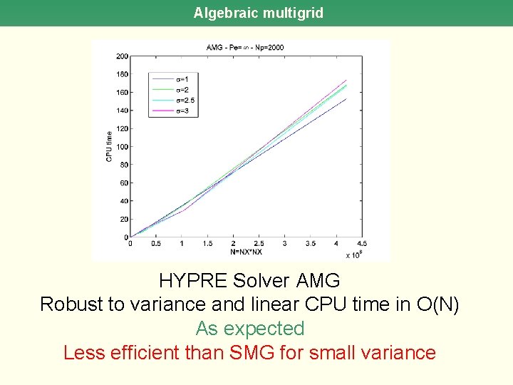
Algebraic multigrid HYPRE Solver AMG Robust to variance and linear CPU time in O(N) As expected Less efficient than SMG for small variance

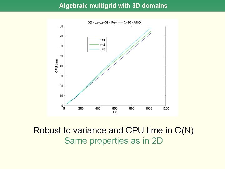
Algebraic multigrid with 3 D domains Robust to variance and CPU time in O(N) Same properties as in 2 D

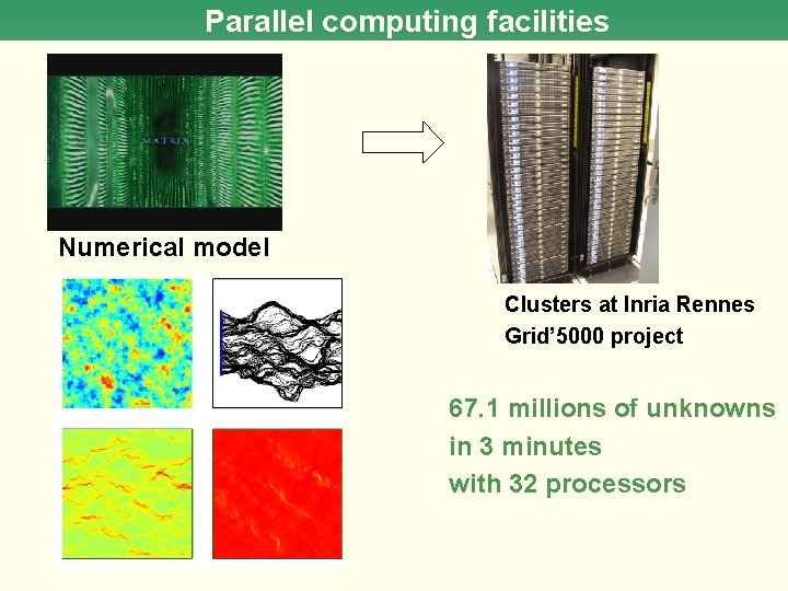
Parallel computing facilities Numerical model Clusters at Inria Rennes Grid’ 5000 project 67. 1 millions of unknowns in 3 minutes with 32 processors

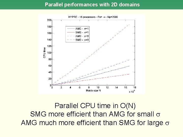
Parallel performances with 2 D domains Parallel CPU time in O(N) SMG more efficient than AMG for small AMG much more efficient than SMG for large

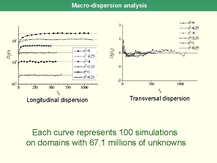
Macro-dispersion analysis Longitudinal dispersion Transversal dispersion Each curve represents 100 simulations on domains with 67. 1 millions of unknowns

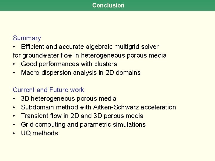
Conclusion Summary • Efficient and accurate algebraic multigrid solver for groundwater flow in heterogeneous porous media • Good performances with clusters • Macro-dispersion analysis in 2 D domains Current and Future work • 3 D heterogeneous porous media • Subdomain method with Aitken-Schwarz acceleration • Transient flow in 2 D and 3 D porous media • Grid computing and parametric simulations • UQ methods